1. Space-time Modelling Using Differential Equations Alan E. Gelfand, ISDS, Duke University (with J. Duan and G. Puggioni)

2. The Contribution Space-time data collection is increasing This talk is entirely about modelling for such data in the case of geo-coded locations Modelling the data directly or using random effects to explain the data Using process models to provide process realizations Using classes of parametric functions to provide realizations Using classes of differential equations to provide realizations

3. Two applications Two examples working with differential equations A realization of a space-time point pattern driven by a random space-time intensity – the application is to urban development measured through housing construction Spatio-temporal data collection - soil moisture measurements in time and space assumed to be a realization of a hydrological model – work in progress

4. Important Points A differential equation in time at every spatial location, i.e., parameters indexed by location The parameters in the differential equation vary spatially as realizations of a spatial process ALTERNATIVELY, the differential equation is a stochastic differential equation (SDE), e.g., a spatial Ornstein-Uhlenbeck process (Brix and Diggle) OR, the rate parameter in the differential equation is assumed to change over time. It can be modelled as a realization of a spatio-temporal process OR, the rate parameter can be modelled using a SDE, yielding an SDE embedded within the differential equation

5. Spatio-temporal Point Process Models Overview: Urban Development & Spatio-temporal Point Processes. Differential Equation Models for Cumulative Intensity Model Fitting & Inference Data Examples: –Simulated data –Urban development data for Irving, TX

6. Urban Development Problem Residential houses in Irving, TX 19511956 19621968

7. Our objectives Space-time point pattern of urban development using a spatio-temporal Cox process model. Work with housing development (available at high resolution) surrogate for population growth (not available at high resolution) Use population models, expect housing dynamics to be similar to population dynamics Differential equation models for surfaces. Insight into interpretable mechanisms of growth Bayesian inference and prediction: –Discretizing time and space(replace integral by sum) –Kernel convolution approximation( to handle large sample size)

8. Spatio-temporal Cox Process In a study region D during a period of [0,T], N T events: Point pattern: is a Poisson process with inhomogeneous intensity Specifying the intensity? are processes for parameters of interest. where

9. The cumulative intensity Discretize the spatio-temporal Cox process in time: during The cumulative intensity foris We consider models for the cumulative intensity Spatial point pattern:

10. Comments

11. Three Growth Models Exponential growth Gompertz growth Logistic growth local growth rate local carrying capacity

12. Logistic Population Growth average growth rate for region D carrying capacity for region D current population at time t population growth at time t Model for the aggregate intensity.

13. Proper Scaling Local growth model should scale with the global growth model: cumulate average

14. Process Models for the Parameters and initial intensity are parameter processes which are modeled on log scale as Hence, given the growth curve is fixed. Also, the μ’s are trend surfaces.

15. Diffusion Model (SDE) for Growth Rate Let Spatial Ornstein-Uhlenbeck (OU) process model: where W t (s) is spatial Brownian motion and, again It induces a stationary process with separable space-time covariance: Can not add scaled spatial Brownian motion to the logistic diff eqn. Instead, a time-varying growth rate at each location

16. Discretizing Time Back to the original model, the intensity for the spatial point pattern in a time interval: Difference equation model: a recursionexplicit transition

17. Discrete-time Model Likelihood Model parameters and latent processes: stochastic integral point i in period j

18. Discretizing Space Divide region D into M cells. Assume homogeneous intensity in each cell. We obtain (with r(m), k(m) average growth rate and cumulative carrying capacity): with induced transition The joint likelihood (product Poisson):

19. Parametrizing the spatial processes Growth rate, carry capacity and initial intensity for each cell: M is very large (2500 in our example) !

20. Kernel Convolution Approximation A dimension reduction approach (2500—>100) Kernel Convolution (Xia & Gelfand, 2006): study region D covering region centroid of block l block l

21. Kernel Convolution Approximation Approximate area of block l centroid of block l kernel function where Let centroid of cell m

22. Kernel Convolution Approximation We use Matérn class covariance function:

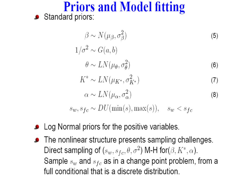
23. Bayesian Inference Posterior: Priors:

24. Bayesian Inference Random-walk Metropolis for posterior exploration: Each parameter is updated sequentially in time in every iteration. are sampled in three blocks.

25. Recursive Calculation Calculate random effects: Sequentially, use

26. Simulated Data Analysis time 0year 1 year 2year 3 Initially and successive 5 years

27. Simulated Data Analysis: Estimation

28. Posterior: Actual: rK

29. Simulation: One Step Ahead Prediction PredictedActual

30. New Houses in Irving, TX: 1952—1957 We use 1951 –1966 to fit our model, leaving 1967 and 1968 out for prediction and validation.

31. Data Analysis for Irving, TX centroid of block l Divide region D into M cells

32. Data Analysis for Irving, TX with points at t 0 rK

33. Prediction: New Houses in1967 & 1968 One Step Ahead 1967 Two Step Ahead 1968

34. Future work on this project Intensity/type of development – marked point pattern Underlying determinants of development, e.g., zoning, roads, time-varying? - add as covariates in rates, carrying capacities Holes, e.g., lakes, parks, externalities – force zero growth Fit the SDE within the DE A model where the observations drive the intensity, e.g., a self-exciting process

35. Conclusion Contributions –Integrate Spatio-temporal point process, Bayesian hierarchical models and SDE models –Urban growth research with high spatial resolution –Directly interpretable results Future Work –SDE model for random growth rate –Better approximation for the likelihood –Need efficient Metropolis-Hasting algorithm

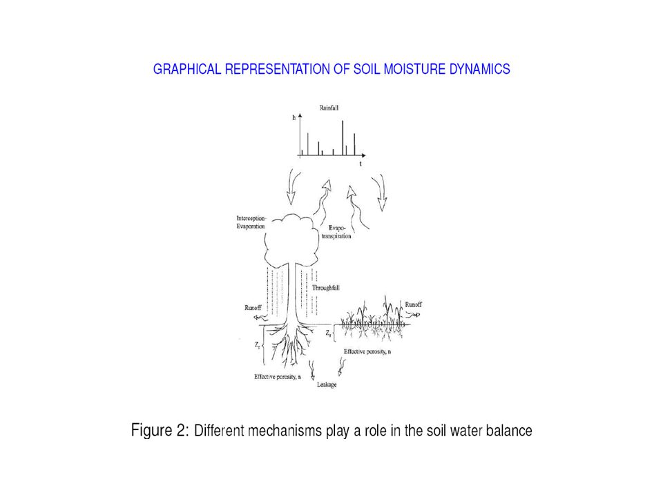
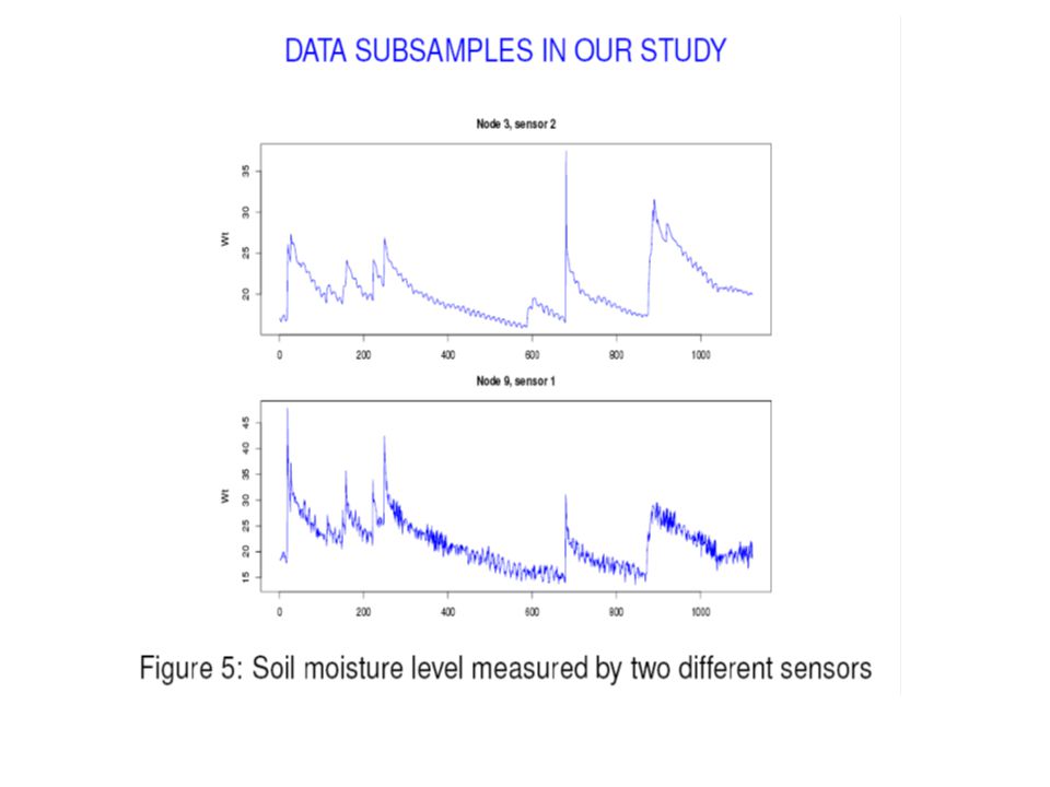
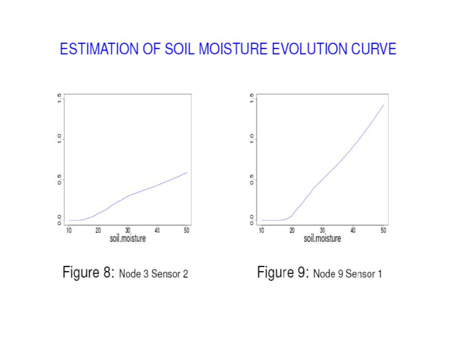
45. Soil moisture loss, i.e., transpiration and drainage as a function of soil moisture

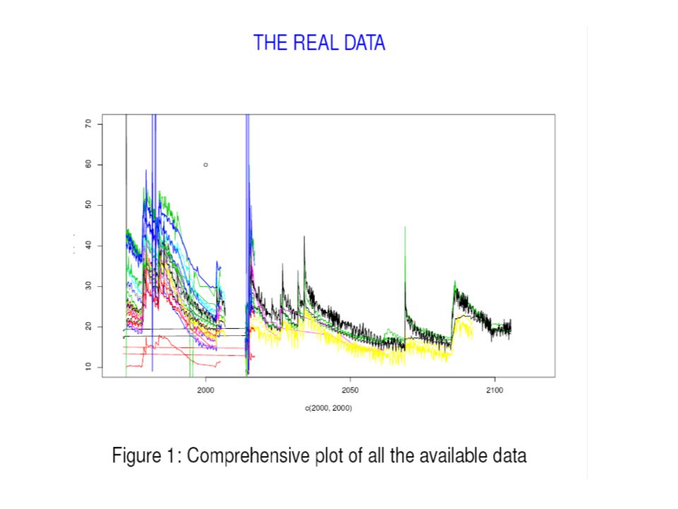
47. A simulated data set

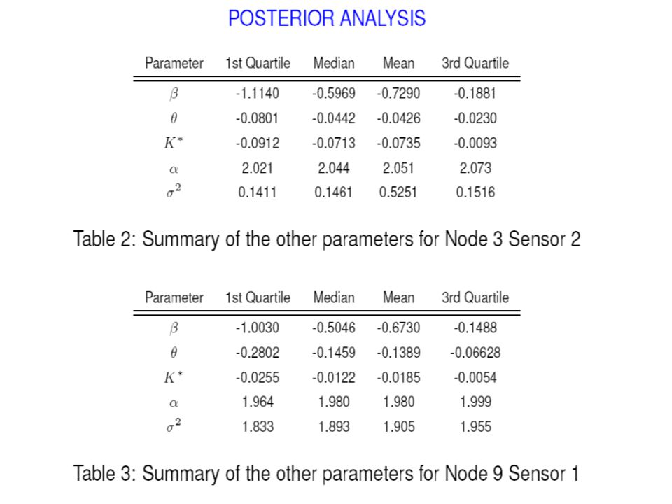
48. Results

50. First Differences

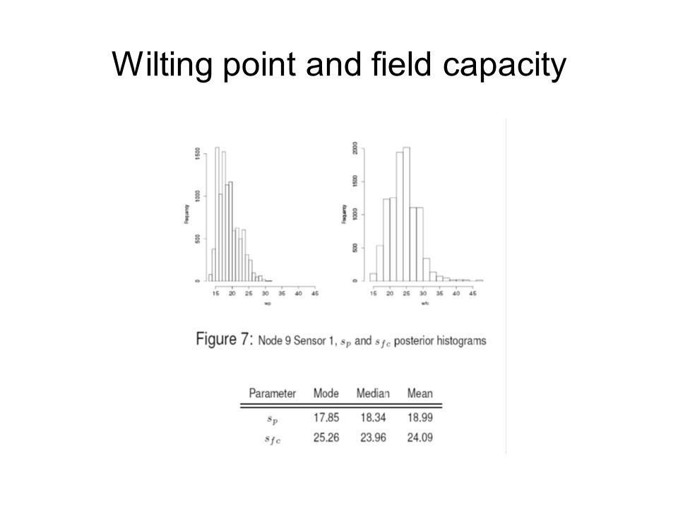
51. Wilting point and field capacity