Download presentation
Presentation is loading. Please wait.

1
Sampling and Reconstruction The impulse response of an continuous-time ideal low pass filter is the inverse continuous Fourier transform of its frequency response Let H lp (jw) be the frequency response of the ideal low-pass filter with the cut-off frequency being w s /2.
 be the frequency response of the ideal low-pass filter with the cut-off frequency being w s /2.")
2
Remember that when we sample a continuous band-limited signal satisfying the sampling theorem, then the signal can be reconstructed by ideal low-pass filtering.

3
The sampled continuous-time signal can be represented by an impulse train: Note that when we input the impulse function (t) into the ideal low-pass filter, its output is its impulse response When we input x s (t) to an ideal low-pass filter, the output shall be It shows that how the continuous-time signal can be reconstructed by interpolating the discrete-time signal x[n].
![The sampled continuous-time signal can be represented by an impulse train: Note that when we input the impulse function (t) into the ideal low-pass filter, its output is its impulse response When we input x s (t) to an ideal low-pass filter, the output shall be It shows that how the continuous-time signal can be reconstructed by interpolating the discrete-time signal x[n].](http://images.slideplayer.com/30/9515213/slides/slide_3.jpg "The sampled continuous-time signal can be represented by an impulse train: Note that when we input the impulse function (t) into the ideal low-pass filter, its output is its impulse response When we input x s (t) to an ideal low-pass filter, the output shall be It shows that how the continuous-time signal can be reconstructed by interpolating the discrete-time signal x[n].")
4
Properties: h r (0) = 1; h r (nT) = 0 for n= 1, 2, …; It follows that x r (mT) = x c (mT), for all integer m. The form sin(t)/t is referred to as a sinc function. So, the interpolant of ideal low-pass function is a sinc function.
/t is referred to as a sinc function. So, the interpolant of ideal low-pass function is a sinc function..")
5
Illustration of reconstruction

6
Ideal discrete-to-continuous (D/C) converter It defines an ideal system for reconstructing a bandlimited signal from a sequence of samples.
 converter It defines an ideal system for reconstructing a bandlimited signal from a sequence of samples.")
7
Ideal low pass filter is non-causal Since its impulse response is not zero when n<0. Ideal low pass filter can not be realized It can not be implemented by using any difference equations. Hence, in practice, we need to design filters that can be implemented by difference equations, to approximate ideal filters.

8
Discrete-time Fourier Transform z-transform: polynomial representation of a sequence Z-Transform

9
Z-transform operator: The z-transform operator is seen to transform the sequence x[n] into the function X{z}, where z is a continuous complex variable. –From time domain (or space domain, n-domain) to the z-domain Z-Transform (continue)
![Z-transform operator: The z-transform operator is seen to transform the sequence x[n] into the function X{z}, where z is a continuous complex variable.](http://images.slideplayer.com/30/9515213/slides/slide_9.jpg "–From time domain (or space domain, n-domain) to the z-domain Z-Transform (continue).")
10
Two sided or bilateral z-transform Unilateral z-transform Bilateral vs. Unilateral

11
Example of z-transform n n 1 012345N>5 x[n]x[n]02464210
![Example of z-transform n n N>5 x[n]x[n]](http://images.slideplayer.com/30/9515213/slides/slide_11.jpg "Example of z-transform n n N>5 x[n]x[n]")
12
If we replace the complex variable z in the z- transform by e jw, then the z-transform reduces to the Fourier transform. The Fourier transform is simply the z-transform when evaluating X(z) only in a unit circle in the z- plane. From another point of view, we can express the complex variable z in the polar form as z = re jw. With z expressed in this form, Relationship to the Fourier Transform
 only in a unit circle in the z- plane. From another point of view, we can express the complex variable z in the polar form as z = re jw. With z expressed in this form, Relationship to the Fourier Transform.")
13
In this sense, the z-transform can be interpreted as the Fourier transform of the product of the original sequence x[n] and the exponential sequence r n. –For r=1, the z-transform reduces to the Fourier transform. Relationship to the Fourier Transform (continue) The unit circle in the complex z plane
![In this sense, the z-transform can be interpreted as the Fourier transform of the product of the original sequence x[n] and the exponential sequence r n.](http://images.slideplayer.com/30/9515213/slides/slide_13.jpg "–For r=1, the z-transform reduces to the Fourier transform. Relationship to the Fourier Transform (continue) The unit circle in the complex z plane.")
14
Relationship to the Fourier Transform (continue) –Beginning at z = 1 (i.e., w = 0 ) through z = j (i.e., w = /2 ) to z = 1 (i.e., w = ), we obtain the Fourier transform from 0 w . –Continuing around the unit circle in the z -plane corresponds to examining the Fourier transform from w = to w = 2 . –Fourier transform is usually displayed on a linear frequency axis. Interpreting the Fourier transform as the z-transform on the unit circle in the z-plane corresponds conceptually to wrapping the linear frequency axis around the unit circle.

15
–The sum of the series may not be converge for all z. Region of convergence (ROC) –Since the z-transform can be interpreted as the Fourier transform of the product of the original sequence x[n] and the exponential sequence r n, it is possible for the z- transform to converge even if the Fourier transform does not. –Eg., x[n] = u[n] is absolutely summable if r>1. This means that the z-transform for the unit step exists with ROC |z|>1. Convergence Region of Z- transform
 –Since the z-transform can be interpreted as the Fourier transform of the product of the original sequence x[n] and the exponential sequence r n, it is possible for the z- transform to converge even if the Fourier transform does not. –Eg., x[n] = u[n] is absolutely summable if r>1. This means that the z-transform for the unit step exists with ROC |z|>1. Convergence Region of Z- transform.")
16
In fact, convergence of the power series X(z) depends only on |z|. If some value of z, say z = z 1, is in the ROC, then all values of z on the circle defined by |z|=| z 1 | will also be in the ROC. Thus the ROC will consist of a ring in the z-plane. ROC of Z-transform

17
ROC of Z-transform – Ring Shape

18
Analytic Function and ROC The z-transform is a Laurent series of z. –A number of theorems from the complex-variable theory can be employed to study the z-transform. –A Laurent series, and therefore the z-transform, represents an analytic function at every point inside the region of convergence. –Hence, the z-transform and all its derivatives exist and must be continuous functions of z with the ROC. –This implies that if the ROC includes the unit circle, the Fourier transform and all its derivatives with respect to w must be continuous function of w.

19
First, we analyze the Z-transform of a causal FIR system –The impulse response is Take the z-transform on both sides Z-transform and Linear Systems nn<00123…MN> M h[n]h[n]0b0b0 b1b1 b2b2 b3b3 …bMbM 0
![First, we analyze the Z-transform of a causal FIR system –The impulse response is Take the z-transform on both sides Z-transform and Linear Systems nn<00123…MN> M h[n]h[n]0b0b0 b1b1 b2b2 b3b3 …bMbM 0](http://images.slideplayer.com/30/9515213/slides/slide_19.jpg "First, we analyze the Z-transform of a causal FIR system –The impulse response is Take the z-transform on both sides Z-transform and Linear Systems nn<00123…MN> M h[n]h[n]0b0b0 b1b1 b2b2 b3b3 …bMbM 0")
20
Z-transform of Causal FIR System (continue) Thus, the z-transform of the output of a FIR system is the product of the z-transform of the input signal and the z-transform of the impulse response.
 Thus, the z-transform of the output of a FIR system is the product of the z-transform of the input signal and the z-transform of the impulse response.")
21
Z-transform of Causal FIR System (continue) H(z) is called the system function (or transfer function) of a (FIR) LTI system. x[n]x[n] y[n]y[n] h[n]h[n] X(z)X(z) Y(z)Y(z) H(z)H(z)
X(z) Y(z)Y(z) H(z)H(z).")
22
Multiplication Rule of Cascading System X(z)X(z) Y(z)Y(z) H1(z)H1(z) Y(z)Y(z) V(z)V(z) H2(z)H2(z) X(z)X(z) Y(z)Y(z) H1(z)H1(z) V(z)V(z) H2(z)H2(z) X(z)X(z) Y(z)Y(z) H1(z)H2(z)H1(z)H2(z)
X(z) Y(z)Y(z) H1(z)H1(z) Y(z)Y(z) V(z)V(z) H2(z)H2(z) X(z)X(z) Y(z)Y(z) H1(z)H1(z) V(z)V(z) H2(z)H2(z) X(z)X(z) Y(z)Y(z) H1(z)H2(z)H1(z)H2(z) ")
23
Example Consider the FIR system y[n] = 6x[n] 5x[n 1] + x[n 2] The z-transform system function is
![Example Consider the FIR system y[n] = 6x[n] 5x[n 1] + x[n 2] The z-transform system function is](http://images.slideplayer.com/30/9515213/slides/slide_23.jpg "Example Consider the FIR system y[n] = 6x[n] 5x[n 1] + x[n 2] The z-transform system function is")
24
Delay of one Sample Consider the FIR system y[n] = x[n 1], i.e., the one- sample-delay system. The z-transform system function is z1z1
![Delay of one Sample Consider the FIR system y[n] = x[n 1], i.e., the one- sample-delay system.](http://images.slideplayer.com/30/9515213/slides/slide_24.jpg "The z-transform system function is z1z1.")
25
Delay of k Samples Similarly, the FIR system y[n] = x[n k], i.e., the k- sample-delay system, is the z-transform of the impulse response [n k]. zkzk
![Delay of k Samples Similarly, the FIR system y[n] = x[n k], i.e., the k- sample-delay system, is the z-transform of the impulse response [n k].](http://images.slideplayer.com/30/9515213/slides/slide_25.jpg "zkzk.")
26
System Diagram of A Causal FIR System The signal-flow graph of a causal FIR system can be re-represented by z-transforms. x[n]x[n] TD x[n-2] x[n-1] x[n-M] + + + + b 1 b 0 b 2 b M y[n]y[n] x[n]x[n] z1z1 z1z1 z1z1 x[n-2] x[n-1] x[n-M] + + + + b 1 b 0 b 2 b M y[n]y[n]

27
Z-transform of General Difference Equation (IIR system) Remember that the general form of a linear constant-coefficient difference equation is When a 0 is normalized to a 0 = 1, the system diagram can be shown as below for all n
 Remember that the general form of a linear constant-coefficient difference equation is When a 0 is normalized to a 0 = 1, the system diagram can be shown as below for all n")
28
Review of Linear Constant- coefficient Difference Equation x[n]x[n] TD x[n-2] x[n-1] x[n-M] + + + + b 1 b 0 b 2 b M + + + + y[n]y[n] TD a 1 a 2 a N y[n-N] y[n-2] y[n-1]
![Review of Linear Constant- coefficient Difference Equation x[n]x[n] TD x[n-2] x[n-1] x[n-M] b 1 b 0 b 2 b M y[n]y[n] TD a 1 a 2 a N y[n-N] y[n-2] y[n-1]](http://images.slideplayer.com/30/9515213/slides/slide_28.jpg "Review of Linear Constant- coefficient Difference Equation x[n]x[n] TD x[n-2] x[n-1] x[n-M] b 1 b 0 b 2 b M y[n]y[n] TD a 1 a 2 a N y[n-N] y[n-2] y[n-1]")
29
Z-transform of Linear Constant- coefficient Difference Equation The signal-flow graph of difference equations represented by z-transforms. X(z)X(z) z1z1 z1z1 z1z1 + + + + b 1 b 0 b 2 b M + + + + Y(z)Y(z) z1z1 z1z1 z1z1 a 1 a 2 a N
X(z) z1z1 z1z1 z1z b 1 b 0 b 2 b M Y(z)Y(z) z1z1 z1z1 z1z1 a 1 a 2 a N.")
30
From the signal-flow graph, Thus, We have Z-transform of Difference Equation (continue)
")
31
Let –H(z) is called the system function of the LTI system defined by the linear constant-coefficient difference equation. –The multiplication rule still holds: Y(z) = H(z)X(z), i.e., Z{y[n]} = H(z)Z{x[n]}. –The system function of a difference equation (or a generally IIR system) is a rational form X(z) = P(z)/Q(z). –Since LTI systems are often realized by difference equations, the rational form is the most common and useful for z- transforms. Z-transform of Difference Equation (continue)
 = H(z)X(z), i.e., Z{y[n]} = H(z)Z{x[n]}. –The system function of a difference equation (or a generally IIR system) is a rational form X(z) = P(z)/Q(z). –Since LTI systems are often realized by difference equations, the rational form is the most common and useful for z- transforms. Z-transform of Difference Equation (continue).")
32
When a k = 0 for k = 1 … N, the difference equation degenerates to a FIR system we have investigated before. It can still be represented by a rational form of the variable z as Z-transform of Difference Equation (continue)
.")
33
When the input x[n] = [n], the z-transform of the impulse response satisfies the following equation: Z{h[n]} = H(z)Z{ [n]}. Since the z-transform of the unit impulse [n] is equal to one, we have Z{h[n]} = H(z) That is, the system function H(z) is the z- transform of the impulse response h[n]. System Function and Impulse Response
![When the input x[n] = [n], the z-transform of the impulse response satisfies the following equation: Z{h[n]} = H(z)Z{ [n]}.](http://images.slideplayer.com/30/9515213/slides/slide_33.jpg "Since the z-transform of the unit impulse [n] is equal to one, we have Z{h[n]} = H(z) That is, the system function H(z) is the z- transform of the impulse response h[n]. System Function and Impulse Response.")
34
Convolution Take the z-transform on both sides: Z-transform vs. Convolution

35
Time domain convolution implies Z-domain multiplication Z-transform vs. Convolution (con’t)
")
36
Generally, for a linear system, y[n] = T{x[n]} –it can be shown that Y{z} = H(z)X(z). where H(z), the system function, is the z-transform of the impulse response of this system T{ }. –Also, cascading of systems becomes multiplication of system function under z-transforms. System Function and Impulse Response (continue) X(z)X(z) Y(z) (= H(z)X(z)) H(z)/H( e jw ) X(e jw ) Y(e jw ) (= H( e jw )X( e jw )) Z-transform Fourier transform
![Generally, for a linear system, y[n] = T{x[n]} –it can be shown that Y{z} = H(z)X(z).](http://images.slideplayer.com/30/9515213/slides/slide_36.jpg "where H(z), the system function, is the z-transform of the impulse response of this system T{ }. –Also, cascading of systems becomes multiplication of system function under z-transforms. System Function and Impulse Response (continue) X(z)X(z) Y(z) (= H(z)X(z)) H(z)/H( e jw ) X(e jw ) Y(e jw ) (= H( e jw )X( e jw )) Z-transform Fourier transform.")
37
Pole: –The pole of a z-transform X(z) are the values of z for which X(z)= . Zero: –The zero of a z-transform X(z) are the values of z for which X(z)=0. When X(z) = P(z)/Q(z) is a rational form, and both P(z) and Q(z) are polynomials of z, the poles of are the roots of Q(z), and the zeros are the roots of P(z), respectively. Poles and Zeros
 are the values of z for which X(z)=0. When X(z) = P(z)/Q(z) is a rational form, and both P(z) and Q(z) are polynomials of z, the poles of are the roots of Q(z), and the zeros are the roots of P(z), respectively. Poles and Zeros.")
38
Zeros of a system function –The system function of the FIR system y[n] = 6x[n] 5x[n 1] + x[n 2] has been shown as The zeros of this system are 1/3 and 1/2, and the pole is 0. Since 0 and 0 are double roots of Q(z), the pole is a second-order pole. Examples
![Zeros of a system function –The system function of the FIR system y[n] = 6x[n] 5x[n 1] + x[n 2] has been shown as The zeros of this system are 1/3 and 1/2, and the pole is 0.](http://images.slideplayer.com/30/9515213/slides/slide_38.jpg "Since 0 and 0 are double roots of Q(z), the pole is a second-order pole. Examples.")
39
Example: Finite-length Sequence (FIR System) Given Then There are the N roots of z N = a N, z k = ae j(2 k/N). The root of k = 0 cancels the pole at z=a. Thus there are N 1 zeros, z k = ae j(2 k/N), k = 1 …N, and a (N 1) th order pole at zero.
, k = 1 …N, and a (N 1) th order pole at zero..")
40
Pole-zero Plot

41
Right-sided sequence: –A discrete-time signal is right-sided if it is nonzero only for n 0. Consider the signal x[n] = a n u[n]. For convergent X(z), we need –Thus, the ROC is the range of values of z for which |az 1 | a. Example: Right-sided Exponential Sequence
, we need –Thus, the ROC is the range of values of z for which |az 1 | a. Example: Right-sided Exponential Sequence.")
42
By sum of power series, There is one zero, at z=0, and one pole, at z=a. Example: Right-sided Exponential Sequence (continue) : zeros : poles Gray region: ROC
 : zeros : poles Gray region: ROC.")
43
Left-sided sequence: –A discrete-time signal is left-sided if it is nonzero only for n 1. Consider the signal x[n] = a n u[ n 1]. –If |az 1 | < 1 or, equivalently, |z| < a, the sum converges. Example: Left-sided Exponential Sequence

44
By sum of power series, There is one zero, at z=0, and one pole, at z=a. Example: Left-sided Exponential Sequence (continue) The pole-zero plot and the algebraic expression of the system function are the same as those in the previous example, but the ROC is different.
 The pole-zero plot and the algebraic expression of the system function are the same as those in the previous example, but the ROC is different..")
45
Hence, to uniquely identify a sequence from its z- transform, we have to specify additionally the ROC of the z-transform. Then Another example: given

46
Thus

48
Consider another two-sided exponential sequence Given Since and by the left-sided sequence example

49
Again, the poles and zeros are the same as the previous example, but the ROC is not.

50
Some Common Z-transform Pairs

51
Some Common Z-transform Pairs (continue)
")
52
Properties of the ROC The ROC is a ring or disk in the z-plane centered at the origin; i.e., 0 r R < |z| r L . The Fourier transform of x[n] converges absolutely iff the ROC includes the unit circle. The ROC cannot contain any poles If x[n] is a finite-length (finite-duration) sequence, then the ROC is the entire z-plane except possible z = 0 or z = . If x[n] is a right-sided sequence, the ROC extends outward from the outermost (i.e., largest magnitude) finite pole in X(z) to (and possibly include) z= .
 sequence, then the ROC is the entire z-plane except possible z = 0 or z = . If x[n] is a right-sided sequence, the ROC extends outward from the outermost (i.e., largest magnitude) finite pole in X(z) to (and possibly include) z= ..")
53
Properties of the ROC (continue) If x[n] is a left-sided sequence, the ROC extends inward from the innermost (i.e., smallest magnitude) nonzero pole in X(z) to (and possibly include) z = 0. A two-sided sequence x[n] is an infinite-duration sequence that is neither right nor left sided. The ROC will consist of a ring in the z-plane, bounded on the interior and exterior by a pole, but not containing any poles. The ROC must be a connected region.
![Properties of the ROC (continue) If x[n] is a left-sided sequence, the ROC extends inward from the innermost (i.e., smallest magnitude) nonzero pole in X(z) to (and possibly include) z = 0.](http://images.slideplayer.com/30/9515213/slides/slide_53.jpg "A two-sided sequence x[n] is an infinite-duration sequence that is neither right nor left sided. The ROC will consist of a ring in the z-plane, bounded on the interior and exterior by a pole, but not containing any poles. The ROC must be a connected region..")
54
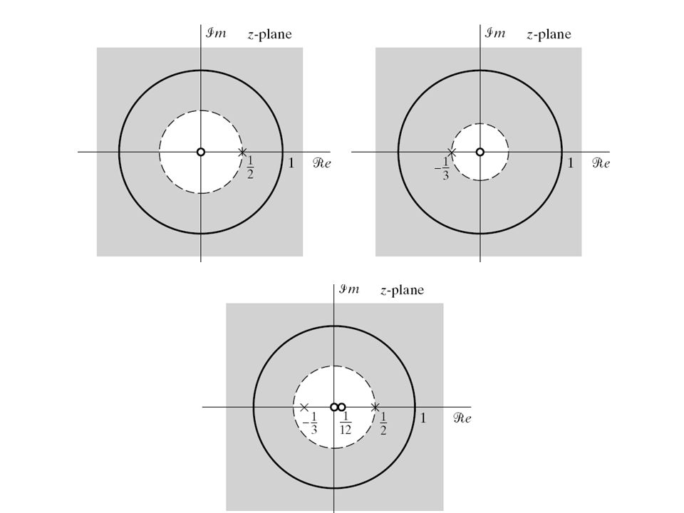
Example A system with three poles

55
Different possibilities of the ROC. (b) ROC to a right- sided sequence. (c) ROC to a left-handed sequence.
 ROC to a left-handed sequence..")
56
Different possibilities of the ROC. (b) ROC to a two-sided sequence. (c) ROC to another two-sided sequence.
 ROC to another two-sided sequence..")
57
ROC vs. Linear System Consider the system function H(z) of a linear system: –If the system is stable, the impulse response h(n) is absolutely summable and therefore has a Fourier transform, then the ROC must include the unit circle,. –If the system is causal, then the impulse response h(n) is right-sided, and thus the ROC extends outward from the outermost (i.e., largest magnitude) finite pole in H(z) to (and possibly include) z= .
 of a linear system: –If the system is stable, the impulse response h(n) is absolutely summable and therefore has a Fourier transform, then the ROC must include the unit circle,. –If the system is causal, then the impulse response h(n) is right-sided, and thus the ROC extends outward from the outermost (i.e., largest magnitude) finite pole in H(z) to (and possibly include) z= ..")
58
Inverse Z-transform Given X(z), find the sequence x[n] that has X(z) as its z-transform. We need to specify both algebraic expression and ROC to make the inverse Z-transform unique. Techniques for finding the inverse z-transform: –Investigation method: By inspect certain transform pairs. Eg. If we need to find the inverse z-transform of From the transform pair we see that x[n] = 0.5 n u[n].
![Inverse Z-transform Given X(z), find the sequence x[n] that has X(z) as its z-transform.](http://images.slideplayer.com/30/9515213/slides/slide_58.jpg "We need to specify both algebraic expression and ROC to make the inverse Z-transform unique. Techniques for finding the inverse z-transform: –Investigation method: By inspect certain transform pairs. Eg. If we need to find the inverse z-transform of From the transform pair we see that x[n] = 0.5 n u[n]..")
59
Inverse Z-transform by Partial Fraction Expansion If X(z) is the rational form with An equivalent expression is
 is the rational form with An equivalent expression is")
60
Inverse Z-transform by Partial Fraction Expansion (continue) There will be M zeros and N poles at nonzero locations in the z-plane. Note that X(z) could be expressed in the form where c k ’ s and d k ’ s are the nonzero zeros and poles, respectively.
 could be expressed in the form where c k ’ s and d k ’ s are the nonzero zeros and poles, respectively..")
61
Inverse Z-transform by Partial Fraction Expansion (continue) Then X(z) can be expressed as Obviously, the common denominators of the fractions in the above two equations are the same. Multiplying both sides of the above equation by 1 d k z 1 and evaluating for z = d k shows that

62
Example Find the inverse z-transform of X(z) can be decomposed as Then
 can be decomposed as Then")
63
Example (continue) Thus From the ROC, we have a right-hand sequence. So
 Thus From the ROC, we have a right-hand sequence. So")
64
Find the inverse z-transform of Since both the numerator and denominator are of degree 2, a constant term exists. B 0 can be determined by the fraction of the coefficients of z 2, B 0 = 1/(1/2) = 2. Another Example
 = 2. Another Example.")
65
From the ROC, the solution is right-handed. So Another Example (continue)
")
66
We can determine any particular value of the sequence by finding the coefficient of the appropriate power of z 1. Power Series Expansion

67
Find the inverse z-transform of By directly expand X(z), we have Thus, Example: Finite-length Sequence
, we have Thus, Example: Finite-length Sequence")
68
Find the inverse z-transform of Using the power series expansion for log(1+x) with |x|<1, we obtain Thus Example
 with |x|<1, we obtain Thus Example")
69
Suppose Linearity Z-transform Properties

70
Time shifting Multiplication by an exponential sequence Z-transform Properties (continue) (except for the possible addition or deletion of z=0 or z= . )
.")
71
Differentiation of X(z) Conjugation of a complex sequence Z-transform Properties (continue)
 Conjugation of a complex sequence Z-transform Properties (continue)")
72
Time reversal If the sequence is real, the result becomes Convolution Z-transform Properties (continue)
")
73
Initial-value theorem: If x[n] is zero for n<0 (i.e., if x[n] is causal), then Inver z-transform formula: Z-transform Properties (continue) Find the inverse z-transform by Integration in the complex domain
![Initial-value theorem: If x[n] is zero for n<0 (i.e., if x[n] is causal), then Inver z-transform formula: Z-transform Properties (continue) Find the inverse z-transform by Integration in the complex domain](http://images.slideplayer.com/30/9515213/slides/slide_73.jpg "Initial-value theorem: If x[n] is zero for n<0 (i.e., if x[n] is causal), then Inver z-transform formula: Z-transform Properties (continue) Find the inverse z-transform by Integration in the complex domain")
74
1.A finite-length sequence is non-zero only at a finite number of positions. If m and n are the first and last non-zero positions, respectively, then we call n m+1 the length of that sequence. What maximum length can the result of the convolution of two sequences of length k and l have? 2.An LTI system is described by the following difference equation: y[n] = 0.3y[n-1] + y[n-2] 0.2y[n-3] + x[n]. Find the system function and frequency response of this system. 3.Find the inverse z-transform of the following system: Homework #2

Similar presentations


 Sogang University Department of Mechanical Engineering.>")


![Z-Transform Fourier Transform z-transform. Z-transform operator: The z-transform operator is seen to transform the sequence x[n] into the function X{z},](/17/5301252/big_thumb.jpg "Z-Transform Fourier Transform z-transform. Z-transform operator: The z-transform operator is seen to transform the sequence x[n] into the function X{z},>")
 Coding and Processing Lecture 2: Basic Filtering Wade Trappe.>")
>")

 Kevin D. Donohue Electrical and Computer Engineering University of Kentucky.>")


![10.0 Z-Transform 10.1 General Principles of Z-Transform linear, time-invariant Z-Transform Eigenfunction Property y[n] = H(z)z n h[n]h[n] x[n] = z n.](/23/6636408/big_thumb.jpg "10.0 Z-Transform 10.1 General Principles of Z-Transform linear, time-invariant Z-Transform Eigenfunction Property y[n] = H(z)z n h[n]h[n] x[n] = z n.>")
