1. Chapter 5: Root Locus Nov. 13-15, 2012

2. Two Conditions for Plotting Root Locus Given open-loop transfer function G k (s) Characteristic equation Magnitude Condition and Argument Condition

3. ContentRules 1Continuity and SymmetrySymmetry Rule 2 Starting and end points Number of segments n segments start from n open-loop poles, and end at m open-loop zeros and (n-m) zeros at infinity. 3Segments on real axisOn the left of an odd number of poles or zeros 4Asymptote n-m segments ： 5Asymptote 3 Rules for Plotting Root Locus

4. 4 7 Angle of emergence and entry Angle of emergence Angle of entry 8Cross on the imaginary axis Substitute s = j  to characteristic equation and solve Routh’s formula 6 Breakaway and break-in points

5. 2016-1-315 Break-in point Breakaway point Rule 6: Breakaway and Break-in Points on the Real Axis Use the following necessary condition

6. 2016-1-316 3. 3.Symmetry5.Asymptote 6.Breakaway and break-in points 4. Segments on real axis 1.Draw the open-loop poles and zeros -2 -3 2. Two segments pole zero breaka way Break- in Example 5.3.1: Given the open-loop transfer function, please draw the root locus. =0.172 =5.818

7. Example 5.3.2: j j  0 s1s1 s2s2 Conclusion: For the open-loop transfer function with one zero and two poles, the root locus of characteristic equation is probably a circle in the complex plane. please prove that the root locus in the complex plane is a circle. Given the open-loop transfer function

8. 2016-1-318 Example 5.3.3: 1.Open-loop poles and zeros  -2 2. Segments on real axis3. Asymptotes 4. Breakaway and break-in points -0.42 5. Points across the imaginary axis K=6 j1.414 K=6 -j1.414

9. 2016-1-319 3. Symmetry 4. No segments on real axis 5. Asymptote6. Breakaway and break-in points 7.The point where the locus across the imaginary axis Example 5.3.4: 1.Find poles and zeros  2. 4 segments Breakaway 484-4 =0 get =121 =121 -j3.16 j3.16 =121

10. Example 5.3.5 Please sketch the root locus with respect to K=[0,+∞).

11. 2016-1-3111 Extension of Root Locus Parameter Root Locus Zero-degree Root Locus Canonical form Root locus gain 1.How to sketch the root locus for other parameters? 2. How to sketch if G k (s)=1 Conventional Root Locus

12. 2016-1-3112 Example 5.3.6: K s is a ramp feedback gain, please sketch the root locus with respect to K s =[0,+∞). 1. Break-in and breakaway point 2. Angle of emergence 90 o 108 o 198 o 5.3.2 Parameter Root Locus

13. 2016-1-3113 Example: Sketch the root loci of the system with the open loop transfer function: 5.3.2 Zero-degree Root Locus Analysis: For this kind of systems, the characteristic equations are like as: Magnitude equation Argument equation

14. 2016-1-3114 Root locus by using the sketching rules with the following modification: Real-axis: Left of even number of zeros or poles Asymptote Angles of emergence and entry For K g varying from － ∞→0 together with K g =[0,+∞) simultaneously, the root loci are named the “complete root loci”.

15. 2016-1-3115 5-4 Application of Root Locus Insert a zero

16. 2016-1-3116 Add a pole to the open-loop transfer function

17. 2016-1-3117 Generally, adding an open zero in the left s-plane will lead the root loci to be bended to the left. The more closer to the imaginary axis the open zero is, the more prominent the effect on the system’s performance is. Generally, adding an open pole in the left s-plane will lead the root loci to be bended to the right. The more closer to the imaginary axis the open pole is, the more prominent the effect on the system’s performance is. 5.4.1 The effects of Zeros and Poles Attracting effect Repelling effect

18. 2016-1-3118 Example 5.4.1: How to enlarge the stability region? 60 o j0.2 ω 1 =0.17 Kc=0.778 -j0.2 ω 2 =-0.17 Kc=0.778 ω 3 =0 Kc=0.278 ω 1 =0 Kc=0.278 -0.06 -0.027

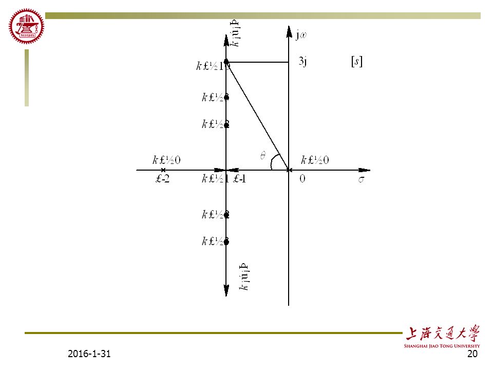
19. 2016-1-3119 5.4.2 Performance Analysis Based on Root Locus Example 5.4.2: Given the open-loop transfer function please analyze the effect of open-loop gain K on the system performance. Calculate the dynamic performance criteria for K ＝ 5.

20. 2016-1-3120

21. 2016-1-3121 It is observed from the root locus that the system is stable for any K. For 0 ＜ K ＜ 0.5(0 ＜ k ＜ 1), there are two different negative real roots. For K=0.5(k=1), there are two same negative real roots. For K ＞ 0.5(k ＞ 1), there are a pair of conjugate complex poles. For K=5( k=10), the closed-loop poles are

22. 2016-1-3122 The criteria for transient performance can be given by Peak time Settling time Overshoot

23. 2016-1-3123 1. We can get the information of the system’s stability by checking whether or not the root loci are on the left half s-plane with the system’s parameter varying. 2. We can get some information of the system’s steady-state error in terms of the number of the open-loop poles at the origin of the s- plane. 3. We can get some information of the system’s transient performance in terms of the tendencies of the root loci with the system’s parameter varying. 4. If the root loci in the left half s-plane move to somewhere far away from the imaginary axis with the system’s parameter varying, the system’s response decays more rapidly and the system is more stable, vice versa.

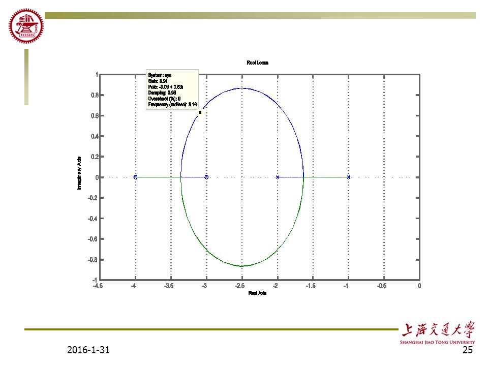
24. Complement Use Matlab to sketch root locus 2016-1-3124 In Matlab: num=[1 7 12] den=[1 3 2] rlocus(num,den) sys=tf[num,den]

25. 2016-1-3125