1. NUAA-Control System Engineering
Chapter 4
Root-locus Technique

2. Contents in Chapter 4 4-1 Introduction 4-2 Root-locus equation
4-3 Rules to draw regular root loci
4-4 Generalized root loci
4-5 Analysis of control system by RL method
4-6 Control system design by the root-locus method 2

3. Introduction
Stability and the characteristics of transient response of closed-loop systems
Locations of the closed-loop poles
Problems to solve characteristic equation :
1. Difficult for a system of third or higher order.
2. Tedious for varying parameters. 3

4. Varying the loop gain K R(s) K Y(s) H(s) G (s) －
The open loop gain K is an important parameter that can affect the performance of a system
In many systems, simple gain adjustment may move the closed-loop poles to desired locations.
Then the design problem may become the selection of an appropriate gain value.
It is important to know how the closed-loop poles move in the s plane as the loop gain K is varied. 4

5. Root locus method
A simple method for finding the roots of the characteristic equation has been developed by W.R.Evans. This method is called root locus method.
Graphical Analysis of Control System, AIEE Trans. Part II,67(1948),pp
Control System Synthesis by Root Locus Method, AIEE Trans. Part II,69(1950),pp.66-69 5

6. The advantages of RL approach:
Root Locus:
the locus of roots of the characteristic equation of the closed-loop system as a specific parameter (usually, gain K) is varied form 0 to ∞.
The advantages of RL approach:
1. Avoiding tedious and complex roots-solving calculation
2. Clearly showing the contributions of each loop poles or zeros to the location of the closed-loop poles.
3. Indicating the manner in which the loop poles and zeros should be modified so that the response meets system performance specifications. 6

7. 4-2 Root-locus equation 7

8. Consider a second-order system shown as follows:
Start from an example
Consider a second-order system shown as follows:
Closed-loop TF:
R(s) -
Y(s)
Characteristic equation (CE):
Roots of CE:
The roots of CE change as the value of k changes.
When k changes from 0 to ∞, how will the locus of the roots of CE move? 8 8

9. k＝0
－1/2 －1
As the value of k increases, the two negative real roots move closer to each other.
A pair of complex-conjugate roots leave the negative real-axis and move upwards and downwards following the line s=-1/2.
On the s plane, using arrows to denote the direction of characteristic roots move when k increases, by numerical value to denote the gain at the poles. 9 9

10. By Root loci, we can analyze the system behaviors
(1)Stability:
when Root loci are on the left half plane, then the system is definitely stable for all k>0.
(2)Steady-state performance:
there ’s an open-loop pole at s=0, so the system is a type I system. The steady-state error is
under step input signal
v0/Kv under ramp signal v0t
∞ under parabolic signal. 10 10

11. (3)Transient performance:
there’s a close relationship between root loci and system behavior
on the real-axis: k<0.25 underdamped;
k=0.25 critically damped
k>0.25 underdamped.
However, it’s difficult to draw root loci directly by closed-loop characteristic roots-solving method.
The idea of root loci : by loop transfer function, draw closed-loop root loci directly.

12. Relationship between zeros and poles of G(s)H(s) and closed-loop ones
R(S)
Y(s)
Forward path TF:
Closed-loop TF:
Feedback path TF: 12

13. Write G(s) and H(s) into zero-pole-gain (zpk) form:
RL gain of forward path
RL gain of feedback path
Zeros of forward path TF
Poles of forward path TF
Zeros of feedback path TF
Poles of feedback path TF

14. 1.The closed-loop zeros = feed forward path zeros + feedback path poles.
2. The closed-loop poles are related to poles and zeros of G(s)H(s) and loop gain K.
3.The closed-loop root loci gain = the feed forward path root loci gain

15. Root-locus equation To draw Closed-loop root locus is to solve the CE
That is
RL equation
Suppose that G(s)H(s) has m zeros (Zi) and n poles（Pi), the above equation can be re-written as
K* varies from 0 to ∞ 15

16. Magnitude equation (ME) Angle equation (AE)
RL equation:
Since G(s)H(s) is function of a complex variable s, the root locus equation can be described by the following two equations:
Magnitude equation (ME)
Angle equation (AE)
用幅角条件来绘制根轨迹，用幅值条件来确定已知根轨迹上某一点K’的值。
Magnitude equation is related not only to zeros and poles of G(s)H(s), but also to RL gain ；
Angel equation is only related to zero and poles of G(s)H(s).
Use AE to draw root loci and use ME to determine the value of K on root loci. 16 16

17. For a point s1 on the root loci, use AE
Example 1
Poles of G(s)H(s)（×）
Zeros of G(s)H(s)（〇）
For a point s1 on the root loci, use AE
Use ME
Angel is in the direction of anti-clockwise 17

18. Unity-feedback transfer function:
Example 2
Unity-feedback transfer function:
One pole of G(s)H(s):
No zero.
Test a point s1 on the negative real-axis
All the points on the negative real-axis are on RL.
Test a point outside the negative real-axis s2=-1-j
All the points outside the negative real-axis are not on RL. 18

19. However, it’s unrealistic to apply such “probe by each point” method.
1. Find all the points that satisfy the Angle Equation on the s-plane, and then link all these points into a smooth curve, thus we have the system root locus when k* changes from 0 to ∞;
2. As for the given k, find the points that satisfy the Magnitude Equation on the root locus, then these points are required closed-loop poles.
However, it’s unrealistic to apply such “probe by each point” method.
W.R. Evans (1948) proposed a set of root loci drawing rules which simplify the our drawing work.

20. 4-3 Rules to draw regular root loci
(suppose the varying parameter is open-loop gain K ) 20

21. Properties of Root Loci
and points of Root Loci
2 Number of Branches on the RL
3 Symmetry of the RL
4 Root Loci on the real-axis
5 Asymptotes of the RL
6 Breakaway points on the RL
7 Departure angle and arrival angle of RL
8 Intersection of the RL with the imaginary axis
9 The sum of the roots and the product of the roots of the closed-loop characteristic equation 21

22. and points
Root loci originate on the poles of G(s)H(s) (for K=0) and terminates on the zeros of G(s)H(s) (as K=∞). RL
Equation:
Magnitude
Equation:
Root loci start from poles of G(s)H(s)
Root loci end at zeros of G(s)H(s). 22

23. 2 Number of branches on the RL
nth-order system, RL have n starting points and RL have n branches RL
Equation:
The order of the characteristic equation is n as K varies from 0 to ∞ ,n roots changen root loci.
For a real physical system, the number of poles of G(s)H(s) are more than zeros，i.e. n > m.
n root loci end at open-loop zeros（finite zeros)；
m root loci end at open-loop zeros（finite zeros)；
（n－m）root loci end at (n－m) infinite zeros. 23

24. 3 Symmetry of the RL
The RL are symmetrical with respect to the real axis of the s-plane.
The roots of characteristic equation are real or complex-conjugate.
Therefore, we only need to draw the RL on the up half s-plane and on the real-axis, the rest can be obtained by plotting its mirror image. 24

25. 4 RL on the Real Axis zero：z1 poles：p1、p2、p3、p4、p5
On a given section of the real axis, RL for k>0 are found in the section only if the total number of poles and zeros of G(s)H(s) to the right of the section is odd.
zero：z1
poles：p1、p2、p3、p4、p5
Pick a test point s1 on [p2，p3] ？
The sum of angles provided by every pair of complex conjugate poles are 360°;
The angle provided by all the poles and zeros on the right of s1 is 180°;
The angle provided by all the poles and zeros on the left of s1 is 0°. 25 25

26. Consider the following loop transfer function
Example
Consider the following loop transfer function
Determine its root loci on the real axis. jw
Poles:
Zeros:
S-plane
Repeated poles: -6 -5 -4 -3 -2 -1
On the right of [-2，-1] the number of real zeros and poles=3.
On the right of [-6，-4], the number of real zeros and poles=7. 26

27. 5 Asymptotes of RL
When n ≠ m, there will be 2|n-m| asymptotes that describe the behavior of the RL at |s|=∞. RL
Equation:
The angles between the asymptotes and the real axis are（i= 0，1，2，… ,n-m-1） ：
The asymptotes intersect the real axis at： 27

28. Consider the following loop transfer function
Example
Consider the following loop transfer function
Determine the asymptotes of its root loci.
3 poles：0、-1、-5
n-m = 3 -1 = 2
1 zero：-4
The asymptotes intersect the real axis at
The angles between the asymptotes and the real axis are 28

29. Consider the following loop transfer function
Example
Consider the following loop transfer function
Determine the asymptotes of its root loci.
4 poles：0、-1+j、-1-j、-4
n-m=4-1=3
1 zero：-1
The asymptotes intersect the real axis at
The angles between the asymptotes and the real axis are 29 29

30. 6 Breakaway points on the RL
Breakaway points on the RL correspond to multi-order roots of the RL equation.
The breakaway points on the RL are determined by finding the roots of dK/ds=0 or dG(s)H(s)=0. 30 30

31. The breakaway point b is the solution of Method－1
Proof：
Suppose the multi-order root is s1，then we have 31

32. Solutions1 is the breakaway point b
(2) divided by (1) yields
Thus Or
Solutions1 is the breakaway point b 32

33. Ruel 4The intersections [-1,0] and[-3,-2] on the real axis are RL.
Example
The poles and zeros of G(s)H(s) are shown in the following figure, determine its root loci. -1 -2 -3 jω σ
Rule 1、2、3
RL have three branches，starting from poles 0、－2、－3，ending at on finite zero －1 and two infinite zeros. The RL are symmetrical with respect to the real axis.
Ruel 4The intersections [-1,0] and[-3,-2] on the real axis are RL.
Rule 5The RL have two asymptotes(n－m＝2)
Rule 6The RL have breakaway points on the real axis (within[-3,-2]) 33 33

34. K corresponding to the breakaway point has the maximum value. Thus
The breakaway point b is the solution of
Method－2
Proof：
Suppose s moves from p2 to p1, if we increase K from zero，K reaches its maximum when s reaches b. Then K decreases and reaches zero at p1.
K corresponding to the breakaway point has the maximum value. Thus 34

35. Rule 1、2、3、4 n=4,m=0 σ Rule 5 Example jω-2
-j4 -4 jω σ j4
Rule 1、2、3、4 n=4,m=0
the RL are symmetrical with respect to the real axis;
the RL have four branches which start from poles 0,-4 and -2±j4 ;
the RL end at infinite zeros;
the intersection [-4,0] on the real-axis is RL
Rule 5
The RL have four asymptotes. 35

36. Rule 6the breakaway point of the RL
Example -2
-j4 -4 jω σ j4
Rule 6the breakaway point of the RL 36

37. 7 Angles of departure and angles of arrival of the RL
The angle of departure or arrival of a root locus at a pole or zero, respectively, of G(s)H(s) denotes the angle of the tangent to the locus near the point. 37

38. Angle of Departure: Pick up a point s1 that is close to p1
Applying Angle Equation (AE)
s1p1
angle of departure θp1 38

39. Angle of Arrival: 39

40. j Consider the following loop transfer function
Example
Consider the following loop transfer function
Determine its RL when K varies from 0 to ∞.
3 poles P1,2=-1(repeated poles) P3=1；1 zero Z1=0，n-m=2。
3 branches ，2 asymptotes -1 j
-0.5 1
Angle of departure: 40

41. 8 Intersection of the RL with the Imaginary Axis
The characteristic equation have roots on the Im-axis and the system is marginally stable.
Intersection of the RL with Im-axis?
Method 1 Use Routh’s criterion to obtain the value of K when the system is marginally stable, the get ω from K.
Method 2 41

42. Consider the following loop transfer function
Example
Determine the intersection of the RL with Im-axis.
Method 1
Closed-loop CE:
Routh’s Tabulation:
Marginally stable:
K =6
Auxiliary equation:
Intersection point: 42

43. Consider the following loop transfer function
Example
Determine the intersection of the RL with Im-axis.
Method 2
Closed-loop CE:
→Closed-loop CE 43

44. Summary of General Rules for Constructing Root Loci
G(s)
H(s) -
R(S)
Y(s)
First, obtain the
characteristic equation (CE)
Then, rearrange the equation so that the parameters of interest appear as the multiplying factor in the form
We sketch the Root Loci when K>0 varies from 0 to ∞.

45. Step 1: Locate the poles and zeros of G(s)H(s) on the s-plane
Step 1: Locate the poles and zeros of G(s)H(s) on the s-plane. The RL start from poles of G(s)H(s) and terminate at zeros (finite zeros or zeros at infinity)
Step 2: Determine the RL on the real-axis. Choose a test point on the real-axis, if the total number of real poles and real zeros to the right of the test is odd, then the test point is on the RL.
Step 3: Determine the asymptotes of RL.
The angles between the asymptotes and the real axis are（i= 0，1，2，… ,n-m-1） ：
The asymptotes intersect the real-axis at：

46. Step 4: Determine the breakaway and break-in points.
The breakaway and break-in points can be determined by finding the roots of
Step 5: Determine the angle of departure (angle of arrival) of the RL from a complex pole (at a complex zero)
Angle of departure from a complex pole pj=
Angle of arrival at a complex zero zk=

47. Step 6: Find the points where the RL may cross the imaginary-axis.
Method 1 Use Routh’s criterion to obtain the value of K when the system is marginally stable, the get ω from K.
Method 2

48. Sketch RL of the closed-loop system when K varies from 0 to ∞.
Example
Consider a unity feedback system with the open-loop transfer function as:
Sketch RL of the closed-loop system when K varies from 0 to ∞.
Solution.
loop TF:
Step 1: Locate the poles and zeros of G(s)H(s) on the s-plane.
loop poles: p1=0, p2=-3, p3,4=-1±j, n=4;
no loop zeros: m=0; 48

49. Step 3: Determine the asymptotes of RL
Step 2: Determine the RL on the real-axis. The section [0,-3] of the real axis are RL.
-0.5
0.5 1
1.5 -1
-1.5 -2
-2.5 -3
Step 3: Determine the asymptotes of RL
The angles between the asymptotes and the real axis are（i= 0，1，2，… ,n-m-1） ：
The asymptotes intersect the real-axis at： 49

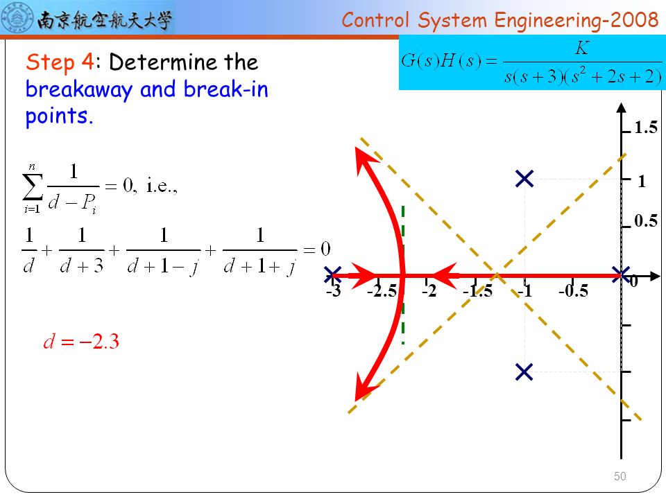
50. Step 4: Determine the breakaway and break-in points.
-0.5
0.5 1
1.5 -1
-1.5 -2
-2.5 -3 50

51. Step 5: Determine the angle of departure (angle of arrival) of the RL from a complex pole (at a complex zero)
-0.5
0.5 1
1.5 -1
-1.5 -2
-2.5 -3
Using measurement to estimate 51

52. Step 6: Find the points where the RL may cross the imaginary-axis.
-0.5
0.5 1
1.5 -1
-1.5 -2
-2.5 -3
The characteristic equation:
Substituting S=jw into the above equation yields: 52

53. The complete RL:
1.5 1
0.5 -3
-2.5 -2
-1.5 -1
-0.5 53

54. RL Demo 1 j j j j j j j j j j j

55. RL Demo 2 j j j j j j j j j j j j

56. Draw RL using MATLAB Loop function: >>n=1;
>>sys=tf(n,d);
>>rlocus(sys) 56

57. Determination of closed-loop poles
Every point on the RL represents a closed-loop pole corresponding to a certain value of K which can be determined according to the Magnitude Equation。
Magnitude Equation :

58. Determine the closed-loop poles when K =4.
Example
Given the RL of a unity feedback system whose open-loop transfer function is:
Determine the closed-loop poles when K =4.
-0.5
0.5 1
1.5 -1
-1.5 -2
-2.5 -3
d＝－2.3
jw＝－1.1

59. Magnitude Equation : Determine the closed-loop pole according to ME:
4 poles，no zero
At the breakaway point d=-2.3, its corresponding K=4.3
K increases from 0 to 4.3
Pick two points within [－3，-2.3] and [-2.3,0] , using trial-and-error to find the closed-loop poles on the real-axis.
So there are exist the two real closed-loop poles locating at two sides of the breakaway point corresponding to K=4

60. Using the ‘Synthetic Division’ to get
Closed-loop CE:
Using the ‘Synthetic Division’ to get

61. So when K=4, the closed-loop transfer function is

62. Effects of Adding Poles and Zeros to G(s)H(s)
Example
Poles: -4, 0 -4 -2
Breakaway point:

63. 1. Addition of poles of G(s)H(s)
Adding a pole to G(s)H(s) has the effect of pushing the root loci toward the right-half plane.
Example
Add a pole at s=-5, we have -5 -4 -3
Poles: -5,-4, 0 no zeros, n=3,m=0 -4 -2
RL on real-axis: (-∞,-5] and [-4,0]
Angle of asymptotes= 60°,180° ,300°
Intersection of asymptotes with real-axis = -3
Breakaway point:
Intersection of RL with Im-axis = ±4.47j

64. 2. Addition of zeros of G(s)H(s)
Adding left-half plane zeros to G(s)H(s) generally has the effect of moving and bending the root loci toward the left-half plane.
Example
Add two zeros at s=-5±3j, we have 3
Poles: -4, 0 zero: -5±3j, n=2,m=2 -4 -2
RL on real-axis: [-4,0] -5 -4 -3
Breakaway point: -3

65. RL for the case of varying zeros of G(s)H(s)
Example 1. Given a system’s structure diagram, where the parameter is speed feedback constant.
Problem: Draw RL when varies from 0 to ∞.
Y(s) s -
R(s)

66. The RL loop transfer function is
Y(s) s -
R(s)
The closed-loop transfer function is：

67. The characteristic equation is:
It can be re-written as
Define
The is the equivalent RL loop transfer function whose RL loop gain is

68. The new system is shown as follows:
The closed-loop transfer function ：
Note: The same denominator, but different numerator, compared with the original system. -
Y(s)
R(s)

69. 2 branches, one approaches to zero, the other approaches to inf
2 poles, 1 zeros
n=2, m=1
For the new system:
2 branches, one approaches to zero, the other approaches to inf
There are RL on the real axis [-∞, 0] jω σ -1 -2 -3 -4 1 2 3

70. Analysis of the influence of variation of Kt on the system
Remark
With the root loci drew by equivalent open-loop transfer function, we can only determine system closed-loop poles, we still need to determine the system closed-loop zeros to analyze system dynamic behavior.
Analysis of the influence of variation of Kt on the system
When Kt varies from 0 to infinity, an zero is added to the loop function G(s)H(s) and the zero moves from the negative infinity to the origin of s-plane.
Y(s) s -
R(s)

71. jω σ -1 -2 -3 -4 1 2 3
When Kt is small, a pair of closed-loop complex-conjugate poles are close to the Im-axis, the overshoot of system step response is large and the oscillation is strong. When Kt is small, the system velocity feedback signal is weak and under-damped.
When Kt increases, the system damp is enhanced, the oscillation is weaken and the overshoot decreases, the system behavior is enhanced.
The breakaway point: Kt＝0.43，the system is critically damped.
When Kt>0.43, the two closed-loop poles are negative and real , the system is over-damped.
Adding left-half plane zeros to open-loop transfer function generally has the effect of moving and bending the root loci toward the left-half s-plane.

72. RL for the case of varying poles of G(s)H(s)
Example 2: Consider a unity feedback system whose open-loop transfer function is
where K and T are given constants,while the parameterτ is to be determined.
Problem: Draw RL whenτvaries from 0 to infinity.

73. The characteristic equation： 1+G(S)H(s)=0
The equivalent open loop transfer function G1(s)：
Solving
Suppose that 4KT>1, then two complex poles of G(S)
are:

74. 2 poles, 3 zeros Z1=Z2=0,Z3=-1/T
So number of branches of the RL is equal to 3.
According to rule 8, the interaction point with the
imaginary axis is determined by 1+G1(jw)=0, that is
It follows that

75. RL whenτvaries from 0 to infinity is shown as follows:
Adding a pole to open-loop transfer function has
The effect of pushing the RL toward the right-half plane
the system is unstable.

76. Consider the RL of a unity-feedback systemj 1 -1 -2
Example
s=0.7j
Consider the RL of a unity-feedback system
k1=0.332
1 Determine the closed-loop TF when its CE has multi-order roots.
d2= -1.37
d1=0.366
k2=13.9
k1=0.0718
2 Determine the steady-state error with a ramp input for underdamped closed-loop system
Solution.
1. RL loop function:
The CE of closed-loop system has multi-order roots at two breakaway points which are actually two closed-loop roots

77. Consider the RL of a unity-feedback systemj 1 -1 -2
Example
s=0.7j
Consider the RL of a unity-feedback system
k1=0.332
1 Determine the closed-loop TF when its CE has multi-order roots.
d2= -1.37
d1=0.366
k2=13.9
k1=0.0718
2 Determine the steady-state error with a ramp input for underdamped closed-loop system
Type-1 system:
Solution.
2. RL loop function:
For a ramp input, the ramp error constant:
Closed-loop system is underdamped:
The steady-state error:

78. An example of a control system analysis and design utilizing Root Locus technique

79. An automatic self-balancing scale

80. We desire to accomplish the following:
Select the parameters of the system
Determine the specifications
Obtain a model represent the system
Design the gain K using root locus
Determine the dominant mode of response

81. Parameters

82. Specifications Specifications
A rapid and accurate response resulting in a small steady-state weight measurement error is desired.
Specifications
Steady-state error (for a step input)
Kp=∞, ess=0
Underdamped response
ζ=0.5
Settling time (error band Δ<2%)
ts<2sec

83. Mathematical model
For a small deviations from balance, the deviation angle is
The motion of the beam about the pivot is represented by the torque equation:

84. Mathematical model The input voltage to the motor is
The transfer function of the motor is:
where τis negligible with respect to the time constants of the overall system and θm is the output shaft rotation.

85. Block diagram
Signal-flow

86. Using Mason’s formula:
The closed-loop transfer function:
Forward path:
Loop path:
The steady-state gain of the system is:
Nontouching loops:
Characteristic equation:

87. Substituting the selected parameter into the CE yields:
To rewrite it into root locus form, first isolate Km as follows:

88. Rewrite it into root locus form:

89. Closed-loop CE:
We draw the root locus as K varies from 0 to ∞
With MATLAB:
> >z=[ i, i];
>>p=[ ];
>>k=1;
>>sys=zpk(z,p,k);
>>rlocus(sys)
The dominant closed-loop poles can be placed at:
To achieve this gain:

90. Let us observe the time-domain step response of the closed-loop system with the designed Km in MATLAB to see if it satisfied the desired specifications.
Specifications
Steady-state error (for a step input)
Kp=∞, ess=0
Underdamped response
ζ=0.5
Settling time (error band Δ<2%)
ts<2sec

91. Parameter Design by Root Locus Technique

92. Originally the root locus method was developed in determine the loci of roots of the characteristic equation as the system gain, K, varies from 0 to ∞.
However, as we have see, the effect of other system parameters may be readily investigated by using the root locus technique.
For example, a third-order equation of interest might be
To ascertain the effect of the parameter α, we isolate the parameter and rewrite the equation in root locus form

93. If there are more than one (m>1) parameters we want to investigate, we must repeat the root locus approach m times.
For example, a third-order characteristic equation with
and as parameters
The effect of varying from 0 to ∞ is determined from the root locus equation
The denominator of the above RL equation is the characteristic equation of the system with

94. Therefore, we must first evaluate the effect of varying
from 0 to ∞ by utilizing
Rewritten as RL form:
Then upon evaluating the effect of , a value of is selected and used to evaluate the effect of .
When more than one parameters varies continuously from 0 to ∞, the family of root loci are referred to as the root contours(RC).

95. Example