Download presentation
Presentation is loading. Please wait.

1
Digital Integrated Circuits A Design Perspective
EE141 Digital Integrated Circuits A Design Perspective Jan M. Rabaey Anantha Chandrakasan Borivoje Nikolic Introduction

2
What is this book all about?
Introduction to digital integrated circuits. CMOS devices and manufacturing technology. CMOS inverters and gates. Propagation delay, noise margins, and power dissipation. Sequential circuits. Arithmetic, interconnect, and memories. Programmable logic arrays. Design methodologies. What will you learn? Understanding, designing, and optimizing digital circuits with respect to different quality metrics: cost, speed, power dissipation, and reliability

3
Digital Integrated Circuits
Introduction: Issues in digital design The CMOS inverter Combinational logic structures Sequential logic gates Design methodologies Interconnect: R, L and C Timing Arithmetic building blocks Memories and array structures

4
Introduction Why is designing digital ICs different today than it was before? Will it change in future?

5
The First Computer

6
ENIAC - The first electronic computer (1946)
")
7
The Transistor Revolution
First transistor Bell Labs, 1948

8
The First Integrated Circuits
Bipolar logic 1960’s ECL 3-input Gate Motorola 1966

9
Intel 4004 Micro-Processor
1971 1000 transistors 1 MHz operation

10
Intel Pentium (IV) microprocessor
 microprocessor")
11
Moore’s Law In 1965, Gordon Moore noted that the number of transistors on a chip doubled every 18 to 24 months. He made a prediction that semiconductor technology will double its effectiveness every 18 months

12
Moore’s Law Electronics, April 19, 1965.

13
Evolution in Complexity

14
Transistor Counts 1 Billion Transistors K 1,000,000 100,000 10,000
Pentium® III 10,000 Pentium® II Pentium® Pro 1,000 Pentium® i486 i386 100 80286 10 8086 Source: Intel 1 1975 1980 1985 1990 1995 2000 2005 2010 Projected Courtesy, Intel

15
Moore’s law in Microprocessors
1000 2X growth in 1.96 years! 100 10 P6 Pentium® proc Transistors (MT) 1 486 386 0.1 286 Transistors on Lead Microprocessors double every 2 years 8086 8085 0.01 8080 8008 4004 0.001 1970 1980 1990 2000 2010 Year Courtesy, Intel
 Transistors on Lead Microprocessors double every 2 years Year. Courtesy, Intel.")
16
Die size grows by 14% to satisfy Moore’s Law
Die Size Growth 100 P6 Pentium ® proc Die size (mm) 486 10 386 286 8080 8086 8085 ~7% growth per year 8008 ~2X growth in 10 years 4004 1 1970 1980 1990 2000 2010 Year Die size grows by 14% to satisfy Moore’s Law Courtesy, Intel
 ~7% growth per year ~2X growth in 10 years Year. Die size grows by 14% to satisfy Moore’s Law. Courtesy, Intel.")
17
Lead Microprocessors frequency doubles every 2 years
10000 Doubles every 2 years 1000 P6 100 Pentium ® proc Frequency (Mhz) 486 10 386 8085 8086 286 1 8080 8008 4004 0.1 1970 1980 1990 2000 2010 Year Lead Microprocessors frequency doubles every 2 years Courtesy, Intel
 Year. Lead Microprocessors frequency doubles every 2 years. Courtesy, Intel.")
18
Lead Microprocessors power continues to increase
Power Dissipation 100 P6 Pentium ® proc 10 486 286 Power (Watts) 8086 386 8085 1 8080 8008 4004 0.1 1971 1974 1978 1985 1992 2000 Year Lead Microprocessors power continues to increase Courtesy, Intel
 Year. Lead Microprocessors power continues to increase. Courtesy, Intel.")
19
Power will be a major problem
100000 18KW 5KW 10000 1.5KW 1000 500W Pentium® proc Power (Watts) 100 286 486 8086 10 386 8085 8080 8008 1 4004 0.1 1971 1974 1978 1985 1992 2000 2004 2008 Year Power delivery and dissipation will be prohibitive Courtesy, Intel
 Year. Power delivery and dissipation will be prohibitive. Courtesy, Intel.")
20
Power density too high to keep junctions at low temp
10000 Rocket Nozzle 1000 Nuclear Reactor Power Density (W/cm2) 100 8086 10 Hot Plate 4004 P6 8008 8085 386 Pentium® proc 286 486 8080 1 1970 1980 1990 2000 2010 Year Power density too high to keep junctions at low temp Courtesy, Intel
 Hot Plate P Pentium® proc Year. Power density too high to keep junctions at low temp. Courtesy, Intel.")
21
Not Only Microprocessors
Analog Baseband Digital Baseband (DSP + MCU) Power Management Small Signal RF RF Cell Phone Digital Cellular Market (Phones Shipped) Units 48M 86M 162M 260M 435M (data from Texas Instruments)
 Power. Management. Small. Signal RF. RF. Cell Phone. Digital Cellular Market. (Phones Shipped) Units 48M 86M 162M 260M 435M. (data from Texas Instruments)")
22
Challenges in Digital Design
µ DSM µ 1/DSM “Microscopic Problems” • Ultra-high speed design Interconnect • Noise, Crosstalk • Reliability, Manufacturability • Power Dissipation • Clock distribution. Everything Looks a Little Different “Macroscopic Issues” • Time-to-Market • Millions of Gates • High-Level Abstractions • Reuse & IP: Portability • Predictability • etc. …and There’s a Lot of Them! ?

23
Complexity outpaces design productivity
Productivity Trends Logic Transistor per Chip (M) 10,000,000 10,000 1,000 100 10 1 0.1 0.01 0.001 100,000,000 0.01 0.1 1 10 100 1,000 10,000 100,000 Logic Tr./Chip 1,000,000 10,000,000 Tr./Staff Month. 100,000 1,000,000 Complexity 58%/Yr. compounded 10,000 (K) Trans./Staff - Mo. Productivity 100,000 Complexity growth rate 1,000 10,000 x x 100 1,000 x x 21%/Yr. compound x x x Productivity growth rate x 10 100 1 10 2003 1981 1983 1985 1987 1989 1991 1993 1995 1997 1999 2001 2005 2007 2009 Source: Sematech Complexity outpaces design productivity Courtesy, ITRS Roadmap
 10,000, ,000. 1, ,000, , , ,000. Logic Tr./Chip. 1,000, ,000,000. Tr./Staff Month. 100,000. 1,000,000. Complexity. 58%/Yr. compounded. 10,000. (K) Trans./Staff - Mo. Productivity. 100,000. Complexity growth rate. 1, ,000. x. x ,000. x. x. 21%/Yr. compound. x. x. x. Productivity growth rate. x Source: Sematech. Complexity outpaces design productivity. Courtesy, ITRS Roadmap.")
24
Why Scaling? Technology shrinks by 0.7/generation
With every generation can integrate 2x more functions per chip; chip cost does not increase significantly Cost of a function decreases by 2x But … How to design chips with more and more functions? Design engineering population does not double every two years… Hence, a need for more efficient design methods Exploit different levels of abstraction

25
Design Abstraction Levels
SYSTEM MODULE + GATE CIRCUIT DEVICE G S D n+ n+

26
Design Metrics How to evaluate performance of a digital circuit (gate, block, …)? Cost Reliability Scalability Speed (delay, operating frequency) Power dissipation Energy to perform a function
 Power dissipation. Energy to perform a function.")
27
Cost of Integrated Circuits
NRE (non-recurrent engineering) costs design time and effort, mask generation one-time cost factor Recurrent costs silicon processing, packaging, test proportional to volume proportional to chip area
 costs. design time and effort, mask generation. one-time cost factor. Recurrent costs. silicon processing, packaging, test. proportional to volume. proportional to chip area.")
28
NRE Cost is Increasing

29
Die Cost Single die Wafer Going up to 12” (30cm)
From

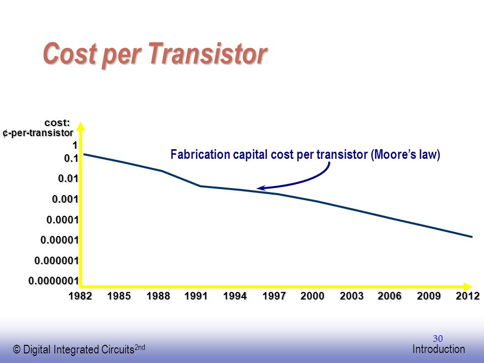
30
Cost per Transistor cost: ¢-per-transistor 1 Fabrication capital cost per transistor (Moore’s law) 0.1 0.01 0.001 0.0001 1982 1985 1988 1991 1994 1997 2000 2003 2006 2009 2012
31
Yield

32
Defects a is approximately 3

33
Some Examples (1994) Chip Metal layers Line width Wafer cost Def./ cm2
Area mm2 Dies/wafer Yield Die cost 386DX 2 0.90 $900 1.0 43 360 71% $4 486 DX2 3 0.80 $1200 81 181 54% $12 Power PC 601 4 $1700 1.3 121 115 28% $53 HP PA 7100 $1300 196 66 27% $73 DEC Alpha 0.70 $1500 1.2 234 53 19% $149 Super Sparc 1.6 256 48 13% $272 Pentium 1.5 296 40 9% $417

34
Reliability― Noise in Digital Integrated Circuits
v ( t ) V DD i ( t ) Inductive coupling Capacitive coupling Power and ground noise
 V. DD. i. ( t. ) Inductive coupling. Capacitive coupling. Power and ground. noise.")
35
DC Operation Voltage Transfer Characteristic
V(x) V(y) V OH OL M f V(y)=V(x) Switching Threshold Nominal Voltage Levels VOH = f(VOL) VOL = f(VOH) VM = f(VM)
 V(y) V. OH. OL. M. f. V(y)=V(x) Switching Threshold. Nominal Voltage Levels. VOH = f(VOL) VOL = f(VOH) VM = f(VM)")
36
Mapping between analog and digital signals
V IL IH in Slope = -1 OL OH out V “ 1 ” OH V IH Undefined Region V IL “ ” V OL

37
Definition of Noise Margins
"1" V OH Noise margin high NM H V IH Undefined Region NM V L Noise margin low IL V OL "0" Gate Output Gate Input

38
Noise Budget Allocates gross noise margin to expected sources of noise
Sources: supply noise, cross talk, interference, offset Differentiate between fixed and proportional noise sources

39
Key Reliability Properties
Absolute noise margin values are deceptive a floating node is more easily disturbed than a node driven by a low impedance (in terms of voltage) Noise immunity is the more important metric – the capability to suppress noise sources Key metrics: Noise transfer functions, Output impedance of the driver and input impedance of the receiver;
 Noise immunity is the more important metric – the capability to suppress noise sources. Key metrics: Noise transfer functions, Output impedance of the driver and input impedance of the receiver;")
40
Regenerative Property
Non-Regenerative

41
Regenerative Property
1 2 3 4 5 6 A chain of inverters Simulated response

42
Fan-in and Fan-out N Fan-out N M Fan-in M

43
The Ideal Gate R = ¥ R = 0 Fanout = ¥ NMH = NML = VDD/2 g = V V i o
in

44
An Old-time Inverter (V) out V 5.0 NM 4.0 3.0 2.0 V NM 1.0 0.0 1.0 2.0
H 1.0 0.0 1.0 2.0 3.0 4.0 5.0 V (V) in
 in.")
45
Delay Definitions

46
Ring Oscillator T = 2 t p N

47
A First-Order RC Network
v out in C R tp = ln (2) t = 0.69 RC Important model – matches delay of inverter
 t = 0.69 RC. Important model – matches delay of inverter.")
48
Power Dissipation Instantaneous power: p(t) = v(t)i(t) = Vsupplyi(t)
Peak power: Ppeak = Vsupplyipeak Average power:

49
Energy and Energy-Delay
Power-Delay Product (PDP) = E = Energy per operation = Pav tp Energy-Delay Product (EDP) = quality metric of gate = E tp
 = E = Energy per operation = Pav tp. Energy-Delay Product (EDP) = quality metric of gate = E tp.")
50
A First-Order RC Network
v out v in CL

51
Summary Digital integrated circuits have come a long way and still have quite some potential left for the coming decades Some interesting challenges ahead Getting a clear perspective on the challenges and potential solutions is the purpose of this book Understanding the design metrics that govern digital design is crucial Cost, reliability, speed, power and energy dissipation

Similar presentations


 Voltage Levels Noise Margins.>")


 Special Topics in Electrical Engineering Low-Power Design of Electronic Circuits.>")

![EE314 Basic EE II Silicon Technology [Adapted from Rabaey’s Digital Integrated Circuits, ©2002, J. Rabaey et al.]](/16/5137281/big_thumb.jpg "EE314 Basic EE II Silicon Technology [Adapted from Rabaey’s Digital Integrated Circuits, ©2002, J. Rabaey et al.]>")


 Circuit Design Presented at ECE1001 Oct. 12th,>")

![EE414 VLSI Design Introduction Introduction to VLSI Design [Adapted from Rabaey’s Digital Integrated Circuits, ©2002, J. Rabaey et al.]](/20/5932086/big_thumb.jpg "EE414 VLSI Design Introduction Introduction to VLSI Design [Adapted from Rabaey’s Digital Integrated Circuits, ©2002, J. Rabaey et al.]>")