Download presentation
Presentation is loading. Please wait.

1
A Myopic History of Great Lakes Remote Sensing
Dr. John R. Schott Digital Imaging and Remote Sensing Laboratory (DIRS) Center for Imaging Science Rochester Institute of Technology
 Center for Imaging Science. Rochester Institute of Technology.")
2
Lake Ontario Comparison of Temperature & Transmission

3
Ontario Mid-lake Temperature Sections
late April mid May early June late June

4
May 25, 1978 ITOS

5
Skylab Photos: chlorophyll maps

6
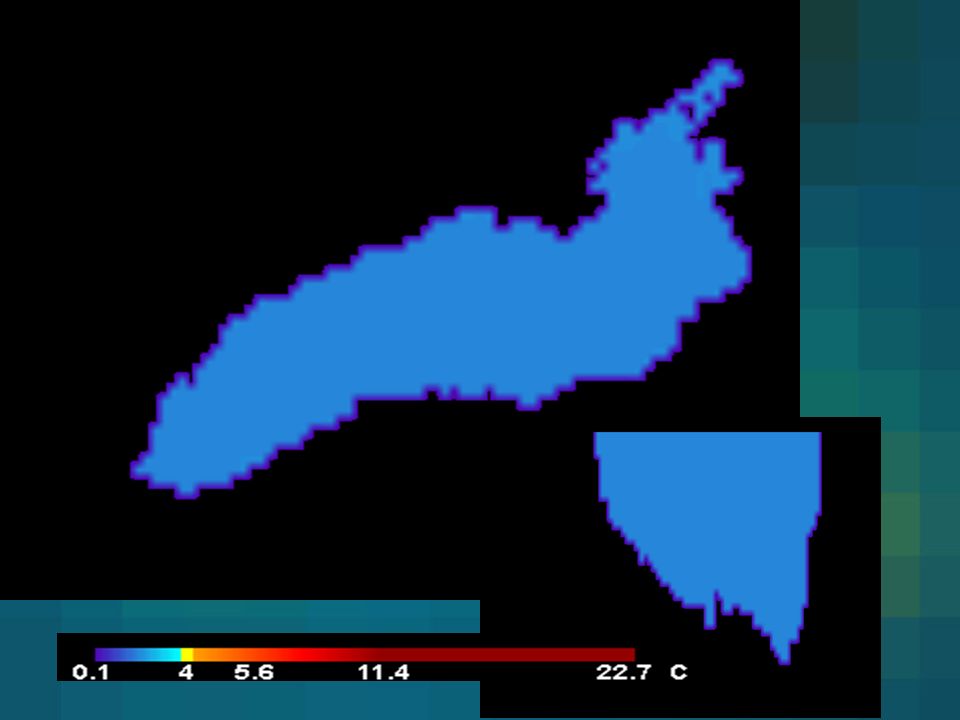
AVHRR Lake Ontario Thermal Bar

7
HCMM Lake Ontario Thermal Bar

8
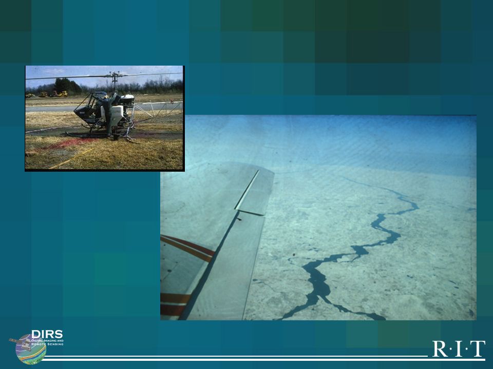
IFYGL Aerial Photos Off Ginna May 22, 1978

9
Landsat Evolution 1972 4 80 m 1982 7 30 m 1999 7 15 m Year
Number of Bands Spot Size Rochester false color infrared true color

10
Landsat TM

11
Landsat TM Ontario Thermal Bar

12
LANDSAT: April 23, 1991 Lakes Ontario & Erie
Cold center Warm ring True Color Composite Thermal Channel

13
Landsat TM April 23, 1991

14
LANDSAT: May 11, 1992 Lakes Ontario & Erie
Cold center Warm ring True Color Composite Thermal Channel

16
Landsat June 12, 1992 True Color Composite Thermal Channel

18
Landsat TM Braddock Bay to True Color Irondequoit Bay Thermal band
Composite (Enhanced) Thermal band warm cold June 23, 1996
 Thermal. band. warm. cold. June 23,")
20
Linking Hydrodynamic Models with Remotely Sensed Data

21
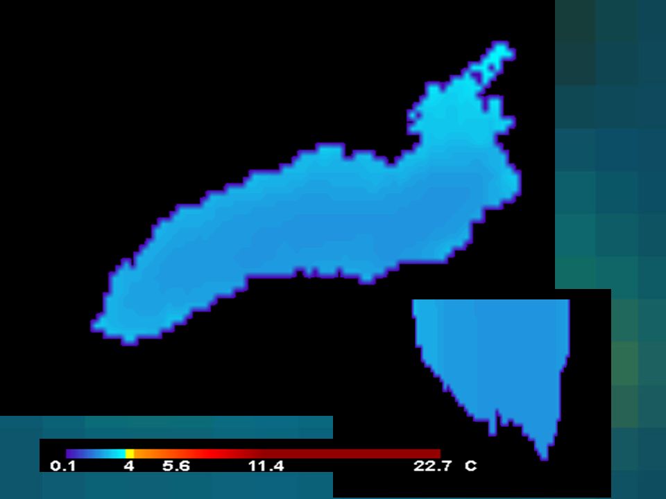
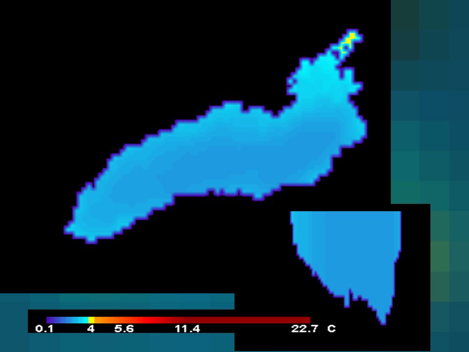
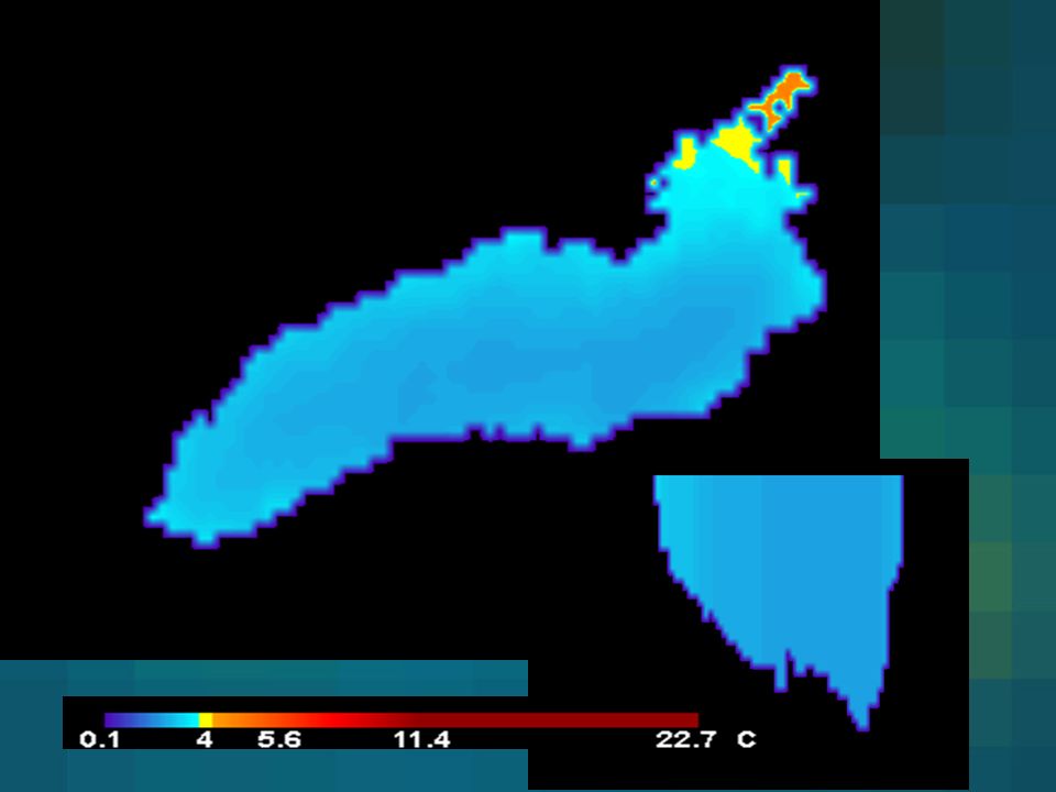
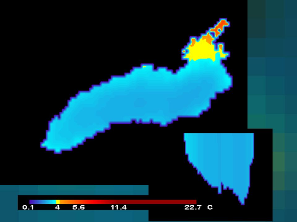
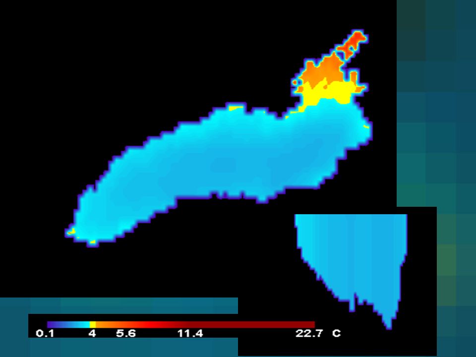
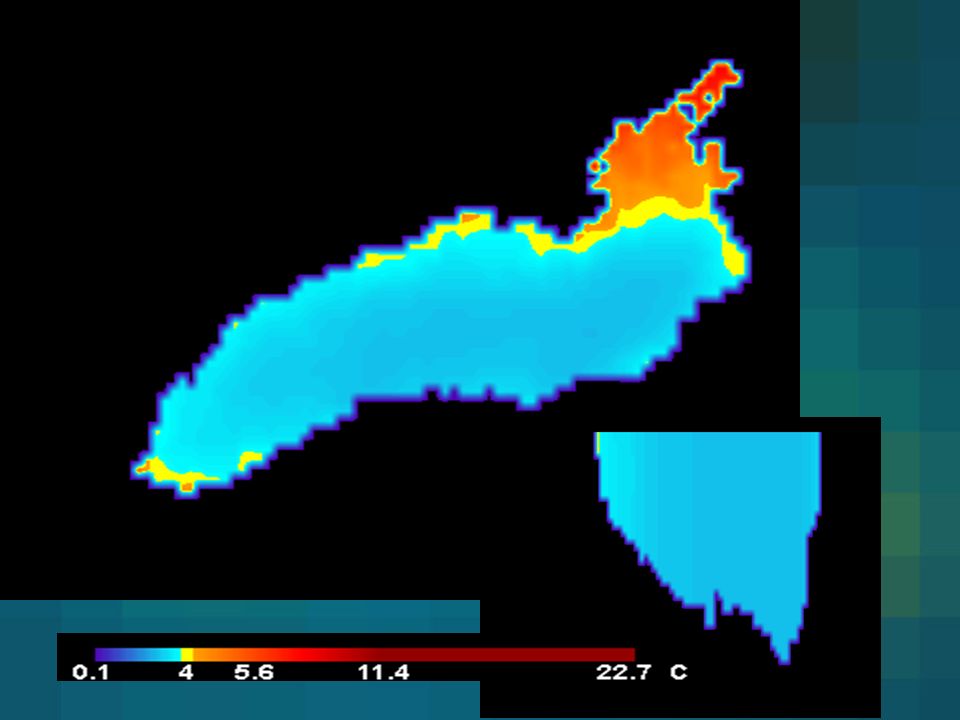
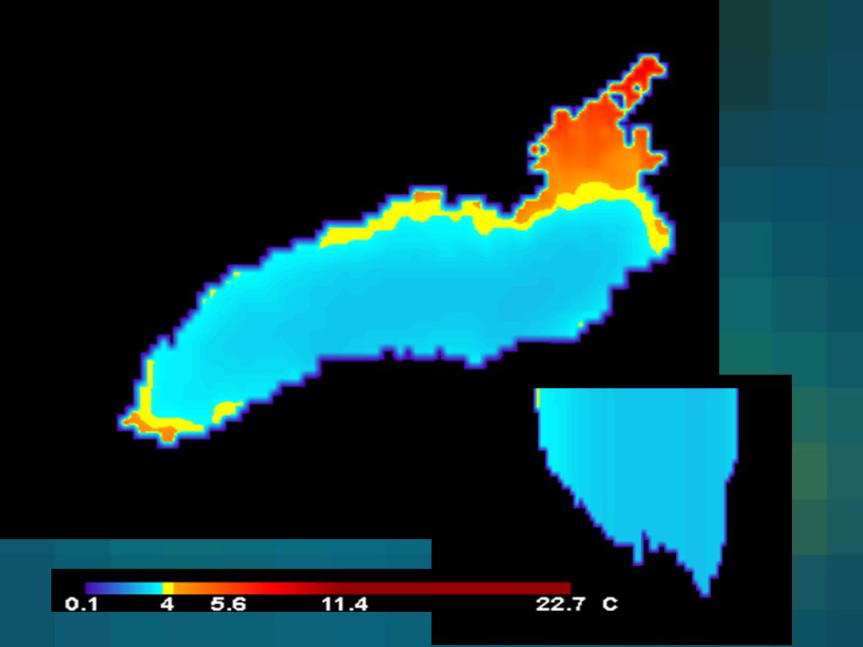
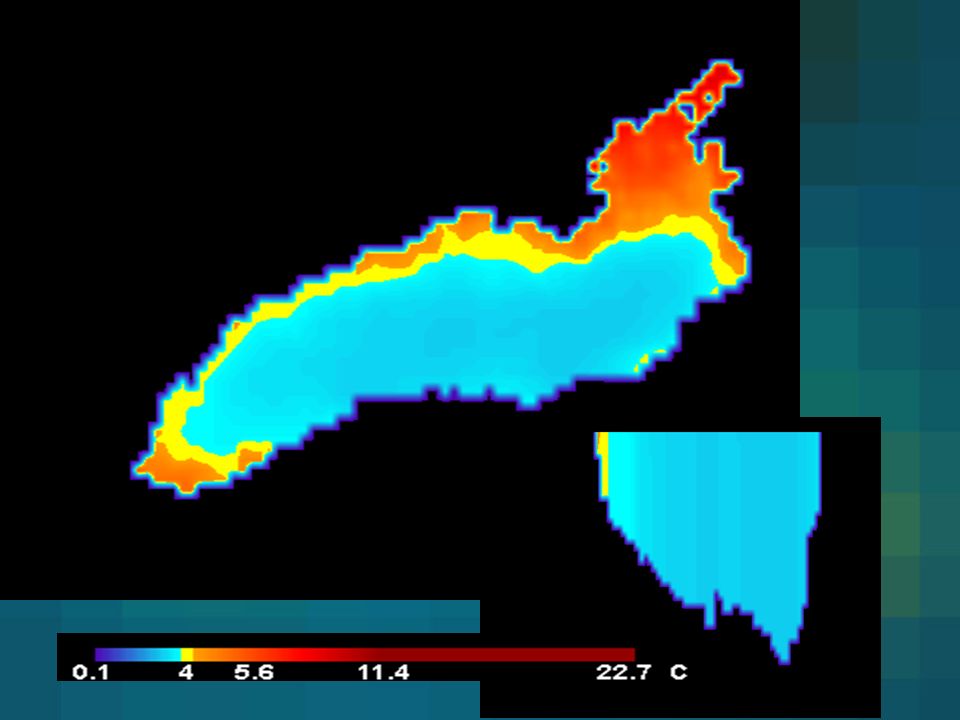
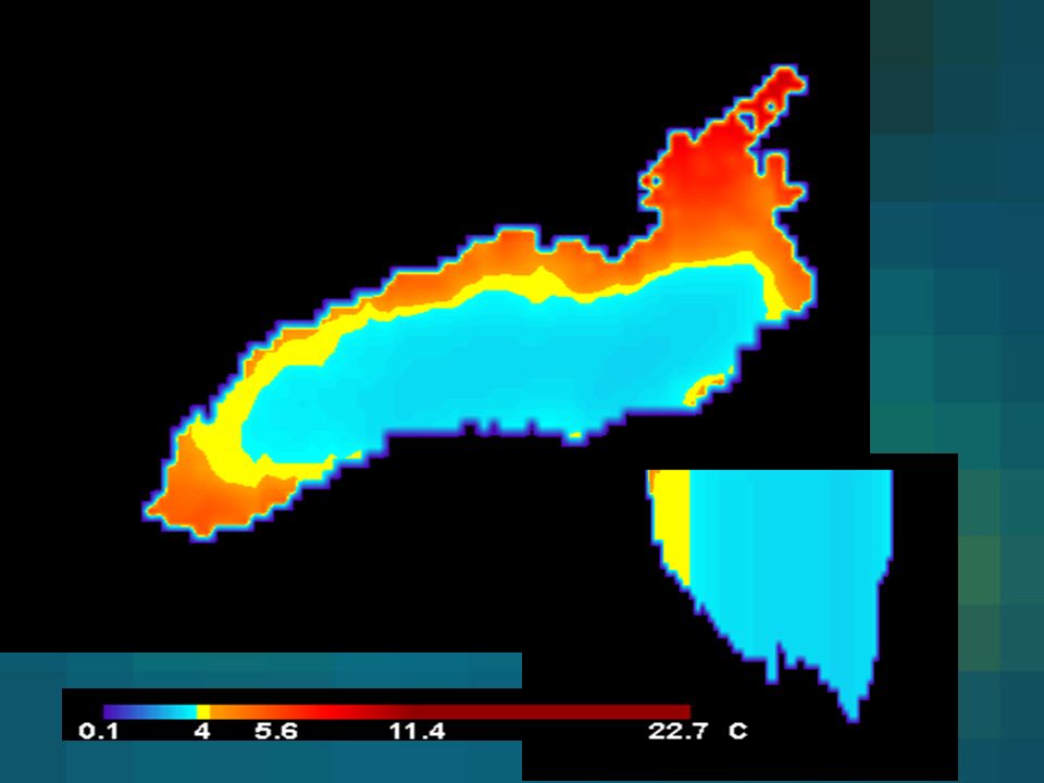
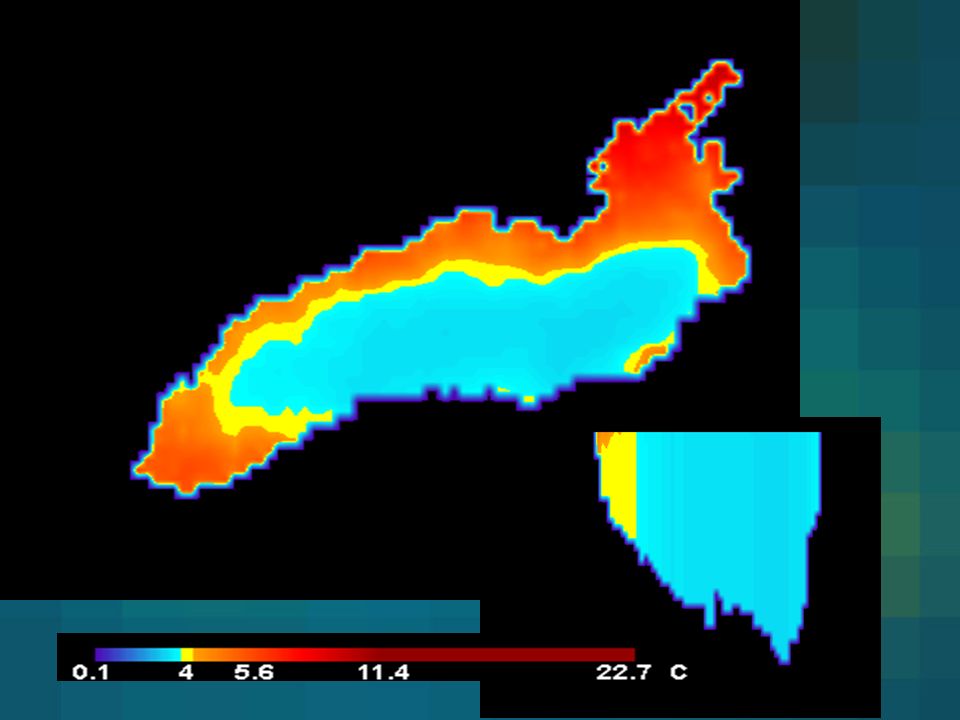
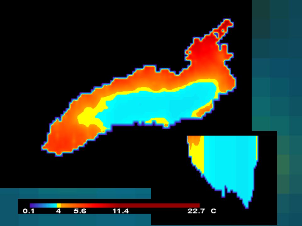
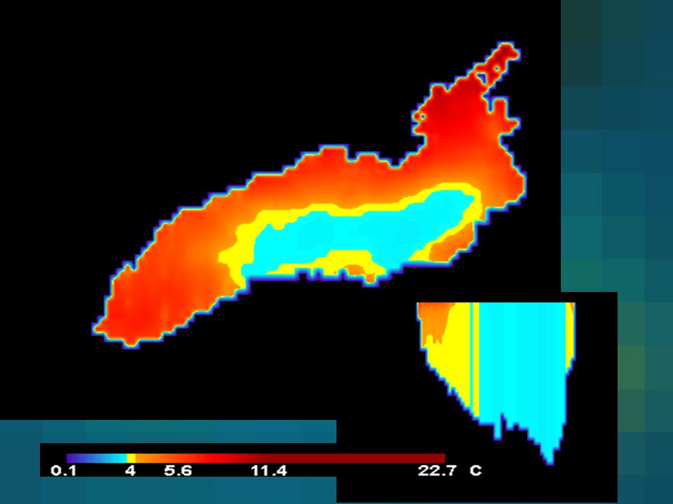
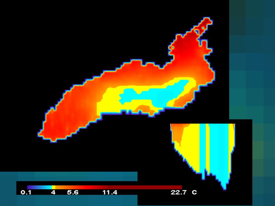
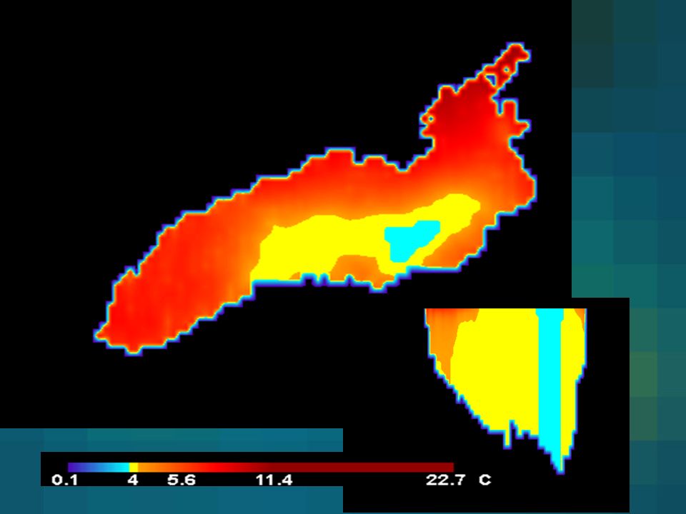
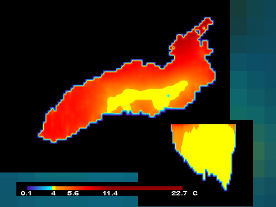
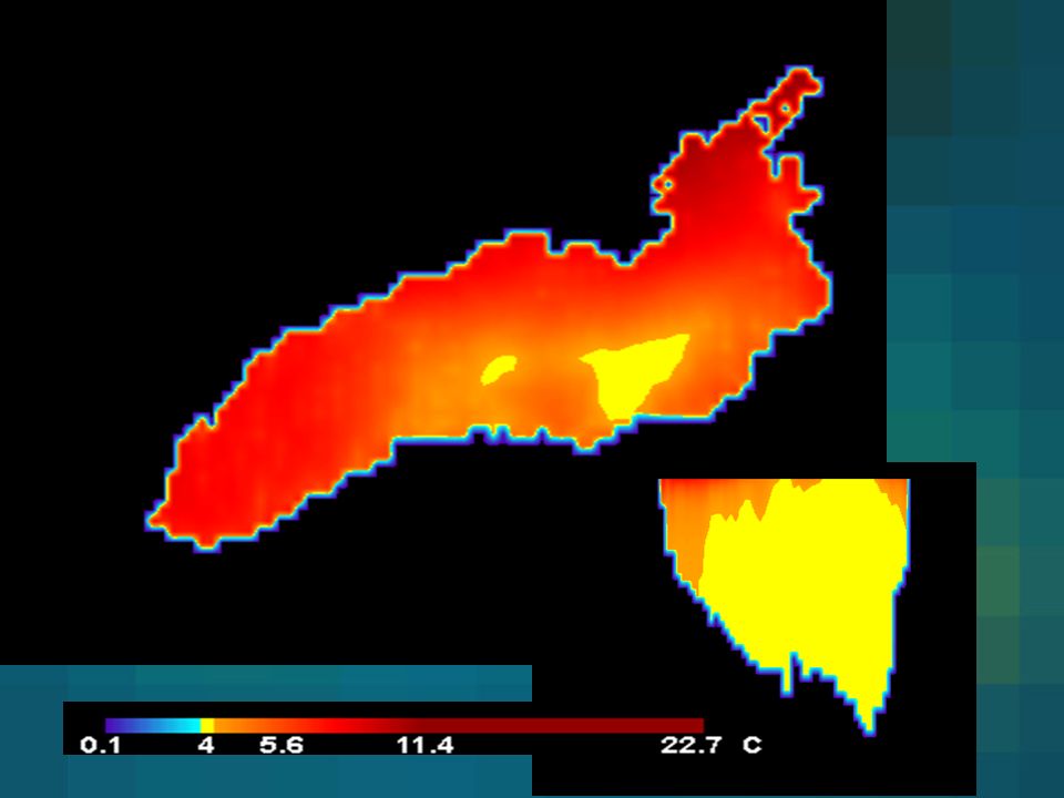
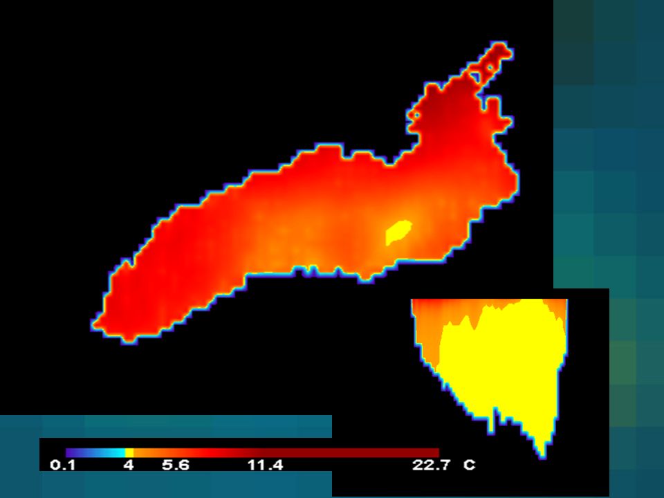
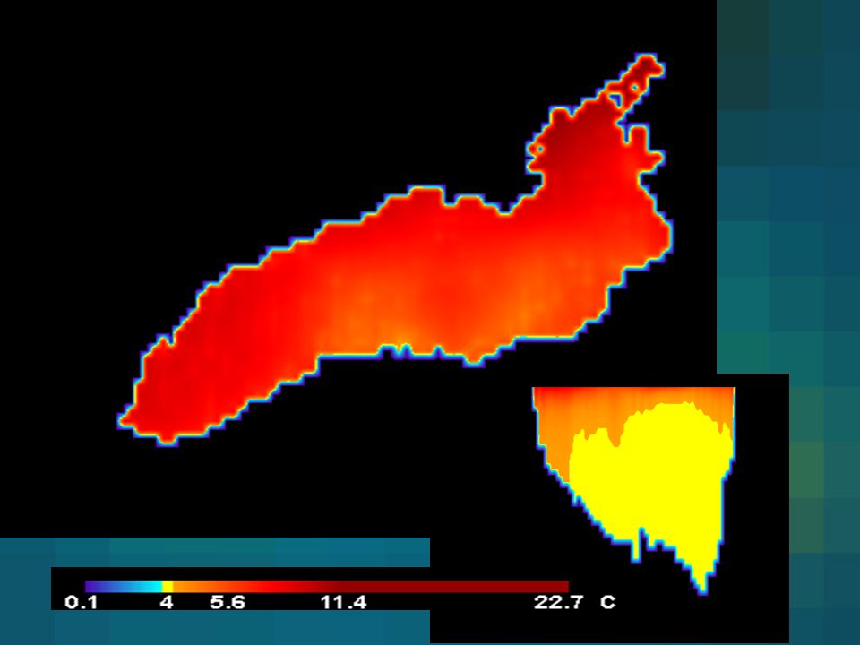
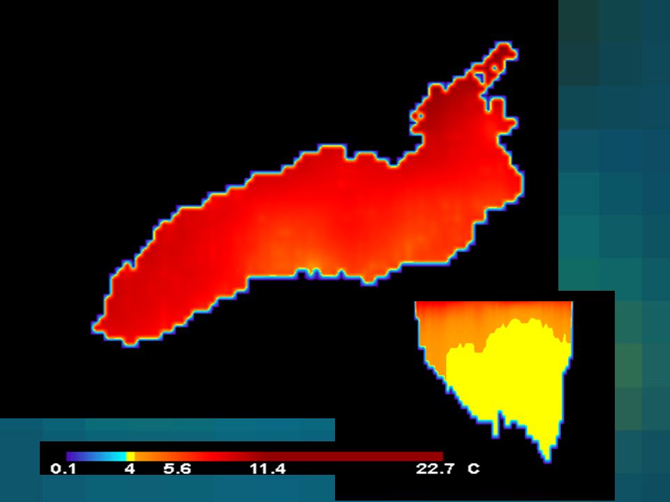
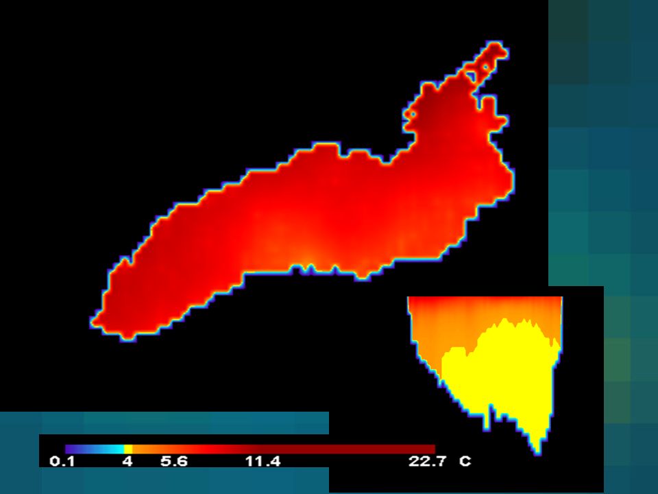
AGLE Simulation including Niagara Inflow
Example outputs of the ALGE 3-D hydrodynamic model with two validation images. The surface temperature map images show the formation and the two phase propagation of the thermal bar (water temperature of C) in Lake Ontario. (Top) Images are for the spring warming conditions after the Niagara inflow and St. Lawrence outflow were added. (Bottom right (2)) Images are east-west cross sections of the lake corresponding to the surface images directly above. (Bottom left (2)) Images are AVHRR derived temperature maps using a different color code and illustrate the need for the incorporation of the Niagara inflow.
 in Lake Ontario. (Top) Images are for the spring warming conditions after the Niagara inflow and St. Lawrence outflow were added. (Bottom right (2)) Images are east-west cross sections of the lake corresponding to the surface images directly above. (Bottom left (2)) Images are AVHRR derived temperature maps using a different color code and illustrate the need for the incorporation of the Niagara inflow.")
22
Hyperspectral Imagery

23
MISI RIT’s Modular Imaging Spectrometer Instrument
Ginna Nuclear Power Plant

24
MISI RIT’s Modular Imaging Spectrometer Instrument
West Roch Embayment Russell Power Plant July 5, 2000 Altitude=4000ft East Roch Embayment Genesee River Plume July 5, 2000 Altitude=4000ft MISI thermal image of Russell Power Plant Effluent

25
Imaging Spectroradiometer
MODIS Moderate Resolution Imaging Spectroradiometer Resolution Trades: Temporal: Global Coverage in 1- 2 days Spatial: 1 km pixels (low) Spectral: 36 bands um
 Spectral: 36 bands um.")
26
MODIS March 5, 2005

27
SeaWiFS April 12, 1998

28
SeaWiFS September 3, 1999

29
Hyperspectral Imagery: AVIRIS
solar glint AVIRIS Flightlines May 20, 1999 11:45 AM Digital Imaging and Remote Sensing Laboratory

30
Hyperspectral Concentration Maps
AVIRIS Image Cube: Lake Ontario Shoreline Provide user community with water quality maps derived from hyperspectral data to address environmental issues. Dr. Rolando Raqueno

31
Spectral Bottom Type Mapping
Dr. Anthony Vodacek AVIRIS May 20, 1999

32
Spectral Bottom Type Mapping
Dr. Anthony Vodacek RIT’s MISI October 1, 2002

33
Comparison of EO-1 and Landsat 7

34
Airborne Hyperspectral Imagery Analysis
Assessing Near Shore Water Quality Airborne Hyperspectral Imagery Analysis Assessing Near Shore Water Quality MODTRAN ALGE Model Agriculture Urban bacteria CDOM phytoplankton HydroLight… macrophytes Modeling Strategy Solar Spectrum Model (MODTRAN) Atmospheric Model (MODTRAN) Air-Water Interface (DIRSIG/Hydrolight) In-Water Model (HYDROMOD= Hydrolight/OOPS + MODTRAN) Bottom Features(HYDROMOD/DIRSIG) particles & algae Bottom Type A Bottom Type B
 Atmospheric Model (MODTRAN) Air-Water Interface (DIRSIG/Hydrolight) In-Water Model (HYDROMOD= Hydrolight/OOPS + MODTRAN) Bottom Features(HYDROMOD/DIRSIG) particles & algae. Bottom Type A. Bottom Type B.")
35
Model of Land/Water Interface What the Future Holds
TopoBathymetry required

36
Where are we going? GIS with satellite derived temporal history of Landuse/Landcover Hydrological models precipitation stream flow materials transport Environmental forcing functions insolation cloud cover wind speed air temperature GL GIS

37
Where are we going? Lakewide Hydrodynamic models with local
and regional inputs temperature and flow models material transport models bio-optical models productivity models driven by temperature, flow, transport, and optical models bio-optical models to predict remotely sensed observables Use of thermal and reflective remote sensing and surface measurements in feedback loops to calibrate models GL GIS HydroMod

38
Future Remote Sensing Trends:
commercial satellites more than just pretty pictures / actual physical earth measurements higher spatial resolution increased spectral resolution/ hyperspectral imaging RS links to models: inputs to climate models verification and validation of models more products available to public IKONOS MODIS AVIRIS MISI

39
ENJOY!!!

40
Airborne Hyperspectral Imagery Analysis Assessing Near Shore Water Quality
Agriculture Urban CDOM bacteria phytoplankton macrophytes particles & algae Bottom Type A Bottom Type B

41
Remote Sensing Platforms: Airborne compared to Satellite
Advanced Very High Resolution Radiometer (1km) Landsat 5 (120m) Landsat 7 (60m) MISI (2-10ft) LANDSAT AVHRR MISI
 Landsat 5 (120m) Landsat 7 (60m) MISI (2-10ft) LANDSAT. AVHRR. MISI.")
42
Coverage vs. Spatial, Spectral, Temporal Resolutions
AVHRR ~1km 1 day Landsat7 30m (vis) 16 day
 16 day.")
43
Chlorophyll Concentration
CZCS Winter

44
Chlorophyll Concentration
CZCS Spring

45
Chlorophyll Concentration
CZCS Summer

46
Chlorophyll Concentration
CZCS Fall

47
Global Biosphere Ocean - CZCS Land - AVHRR

48
Chernobyl, Russia Landsat April 29, 1986

49
Thermal Patterns in Reactor Cooling Pond
April 22, 1986 plant in normal use, pond is warm May 8, 1986 pond in ambient, no activity April 29, 1986 pond cooling, little or no activity

50
Gulf Stream Composite Thermal Patterns
Great Lakes and Western Atlantic

51
Gulf Stream HCMM thermal Urban heat islands New York City Philadelphia
Baltimore Washington

52
Great Lakes Hydrodynamics
A story based on only two graphs... Understanding & Monitoring water quality & flow R.I.T 52 Digital Imaging and Remote Sensing Laboratory

53
Maximum Density of Water

54
Colors of Light Solar Irradiance Outside Earth’s Atmosphere: Transmission of the : Earth’s Atmosphere : Radiant Exitance of Earth Humans can see in the visible region These are mostly reflected photons from the Sun, Moon or lights. Some animals can see in the near infrared (NIR) region This gives them improved contrast of prey against vegetation. Some sensors can “see” in the long-wave infrared (LWIR) This allows them to measure temperatures without touching it.
 region. This gives them improved contrast of prey against vegetation. Some sensors can see in the long-wave infrared (LWIR) This allows them to measure temperatures without touching it.")
55
Great Lakes of the World

56
Great Lakes Profile (Bathymetry & Flow)
Sea Level 229 m 282 m 244 m 406 m Superior Michigan Huron Erie Ontario modified from The Great Lakes Atlas, 1995

57
Laurentian Great Lakes
Hold 18% of the world’s fresh water US coast line exceeds US Atlantic coast About 10% of US and 32% of Canadian population (about 35 million people) live in the Laurentian Basin Large fraction of the industrial northeast
 live in the Laurentian Basin. Large fraction of the industrial northeast.")
58
Seasons of a Dimictic Lake

59
Thermal Stratification & Mixing in a Dimictic Lake
winter stratification spring mixing summer stratification fall mixing

60
Summer Stratification
Thermal Bar Process Lake cross-section Thermal Bar Density Temperature (Celsius) maximum density Summer Stratification Winter Stratification
 maximum density. Summer Stratification. Winter. Stratification.")
61
Thermal Bar Spring Progression Lake Ontario Cross-Sections
Late April Mid May Early June Late June

62
Lake Ontario Comparison of Temperature & Transmission

64
Can Remote Sensing Help?
Can we ‘see’ : Water quality Hydrodynamic processes that impact water quality and materials transport Impact of global / regional forcing functions

65
Questions When does the thermal bar occur? How long does it last?
What functions drive the start, progression and end? Can we predict these occurrences? How does it effect water quality?

66
Hydrodynamic Model to Predict this Thermal Bar Phenomenon

67
Temperature Maps from Hydrodynamic Model
Thermal Bar at 4 Celsius N S N S vertical cross-section Digital Imaging and Remote Sensing Laboratory

68
ALGE Simulation without Niagara inflow
0C 4C 11C 22C Example outputs of the ALGE 3-D hydrodynamic model with two validation images. The surface temperature map images show the formation and the two phase propagation of the thermal bar (water temperature of C) in Lake Ontario. (Top) Images are for the spring warming conditions before the Niagara inflow and St. Lawrence outflow were added. (Bottom right (2)) Images are east-west cross sections of the lake corresponding to the surface images directly above. (Bottom left (2)) Images are AVHRR derived temperature maps using a different color code and illustrate the need for the incorporation of the Niagara inflow.
 in Lake Ontario. (Top) Images are for the spring warming conditions before the Niagara inflow and St. Lawrence outflow were added. (Bottom right (2)) Images are east-west cross sections of the lake corresponding to the surface images directly above. (Bottom left (2)) Images are AVHRR derived temperature maps using a different color code and illustrate the need for the incorporation of the Niagara inflow.")
105
Niagara River: localized plume study
6 hours 12 hours 18 hours 24 hours

106
ALGE simulation including variable inflow at Niagara (March-August 1998)
")
107
ALGE simulation including variable inflow at Niagara (March-August 1998)
")
108
ALGE simulation including variable inflow at Niagara (March-August 1998)
")
109
ALGE simulation including variable inflow at Niagara (March-August 1998)
")
110
ALGE simulation including variable inflow at Niagara (March-August 1998)
")
111
ALGE simulation including variable inflow at Niagara (March-August 1998)
")
112
ALGE simulation including variable inflow at Niagara (March-August 1998)
")
113
ALGE simulation including variable inflow at Niagara (March-August 1998)
")
114
4D Hydrodynamic Modeling
Reference: Schott, de Alwis, Raqueno, Barsi. “Calibration of a Great Lake Hydrodynamic Model Using Remotely Sensed Imagery,” presented at the International Association for Great Lakes Research 43rd Conference on Great Lakes and St. Lawrence River Research, Cornwall, Ontario, May, 2000 Thesis: de Alwis. Simulation of the formation and propagation of the thermal bar on Lake Ontario. RIT, M.S. Thesis, 1999.

115
Landsat TM April 7, 1991

Similar presentations


 Turquoise = phytoplankton bloom.>")


>")


 and Landsat Thematic Mapper (TM) Sensor System Characteristics.>")


-Polar Orbiting Environmental Satellite (POES) Orbital characteristics.>")

 Latitude, Elevation, Global Winds, Proximity to Water, Ocean Currents.>")