1. More on Demand-Supply relationships

2. Demand  Demand relationships are typically drawn in two dimensions D = F(P)  In reality, demand is a functions of several dimensions D = F(P,price of substitutes, price of complements, income, etc.)

3. Demand relationship  The relationships of variable relative to quantity demand is view in term of elasticity Percentage Change in quantity demanded Percentage change in price

4. Demand P Q Elastic Demand E p < -1 Elastic Demand -1<E p < 0 E p = 0

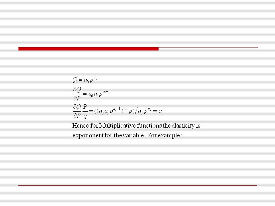
6. Constant Elasticity

7. Demand and Need  Demand and need are not the same  Need is subjective and implies knowledge of requirement  Peterson and Smith equation for low income and elderly need for demand responsive transit

8. Supply in Completitive Market Supplier a Supplier b Supplier c Supplier d Total Market p SRMC SRAC SRMC SRAC SRMC SRAC Market Demand Market Supply qaqa qbqb qcqc Q

9. Supply  Where there are several suppliers, the market is the sum of individual producers.  In transportation supply modeling, the supply is generally one facility and is the same at the cost curve.  Problem is that every one always pays the average cost.

10. Example of miss-allocation QmQm Flow Speed KmKm KmKm KjKj QmQm Density Flow UmUm Unstable Flow

11. Oklahoma City Central Expressway  $80 million per mile or a capital cost of $4.1 million per mile per year  Capital plus operating cost per year $5 million per mile  8 lane facility and 1.5 hours per peak period when 4 th lane in each direction is used (in either direction)  7.5 hours per week or 375 hours per year

12. Example continued ($5mill/8)(1/375)=$1,667 per Lane Mile per hour Assume an hourly flow of 1,700 vehicles per hour Yearly cost 1,667/1,700 = $0.98 per vehicle per mile What the user pays Registration ~ $100/year=100/12,000 miles= $0.0083/mile

13. Example continued  Gas taxes (in 1988) Federal tax – $0.08 per gallon (in highway fund) State tax - $0.12 per gallon (a guess) Total gas tax $0.20 per gallon Gas tax per mile 0.20/20 gpm = 1 cent per mile Total tax – almost 2 cents per mile Deficit is almost $1 per mile

14. FYI Current state gas taxes

15. Marginal Cost Pricing D D A D G B F1F1 F2F2 P’ P SRMC SRAC LRAC

16. Implications of pricing  Social optimum – marginal benefit = marginal cost = price  Social costs of Improper pricing = AGF 1 F 2  Increased Consumer surplus due to improper pricing = ABD  Net loss = AGD (dead weight loss)

17. Difficulties with pricing  Privacy  Estimating demand elasticities  Distribution Effects Unfairly penalizes low income individual and benefits the rich Middle-class will be priced off the highway on transit, thus requiring better service and improving the welfair of the rich (still in cars) and the poor (using transit)

18. Pricing schemes  Roadway user Electronic tolls Physical toll facilities Area licensing  Vehicle use Parking charges On-vehicle meter Annual VMT Charges Fuel use taxes  Vehicle ownership based Vehicle sales taxes – purchasing fees License fees - registration

19. Regulatory schemes  Direct capacity constraints Traffic meters  Direct use regulation Hierarchical network use right Time and place restrictions Work force staggering Vehicle occupancy regulation  Land use regulation Parking supply restrictions Development density regulations Transit service area development