Download presentation
Presentation is loading. Please wait.

1
The Frequency Domain 15-463: Computational Photography Alexei Efros, CMU, Fall 2010 Somewhere in Cinque Terre, May 2005 Many slides borrowed from Steve Seitz

2
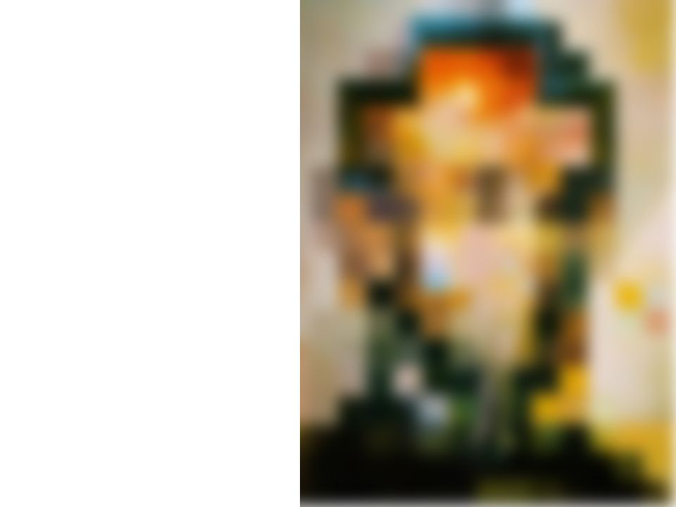
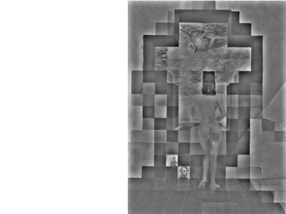
Salvador Dali, “Gala Contemplating the Mediterranean Sea, which at 30 meters becomes the portrait of Abraham Lincoln”, 1976 Salvador Dali “Gala Contemplating the Mediterranean Sea, which at 30 meters becomes the portrait of Abraham Lincoln”, 1976

5
A nice set of basis This change of basis has a special name… Teases away fast vs. slow changes in the image.

6
Jean Baptiste Joseph Fourier (1768-1830) had crazy idea (1807): Any periodic function can be rewritten as a weighted sum of sines and cosines of different frequencies. Don’t believe it? Neither did Lagrange, Laplace, Poisson and other big wigs Not translated into English until 1878! But it’s true! called Fourier Series

7
A sum of sines Our building block: Add enough of them to get any signal f(x) you want! How many degrees of freedom? What does each control? Which one encodes the coarse vs. fine structure of the signal?

8
Fourier Transform We want to understand the frequency of our signal. So, let’s reparametrize the signal by instead of x: f(x) F( ) Fourier Transform F( ) f(x) Inverse Fourier Transform For every from 0 to inf, F( ) holds the amplitude A and phase of the corresponding sine How can F hold both? Complex number trick! We can always go back:
 F( ) Fourier Transform F( ) f(x) Inverse Fourier Transform For every from 0 to inf, F( ) holds the amplitude A and phase of the corresponding sine How can F hold both. Complex number trick. We can always go back:.")
9
Time and Frequency example : g(t) = sin(2pf t) + (1/3)sin(2p(3f) t)
 = sin(2pf t) + (1/3)sin(2p(3f) t)")
10
Time and Frequency example : g(t) = sin(2pf t) + (1/3)sin(2p(3f) t) = +
 = sin(2pf t) + (1/3)sin(2p(3f) t) = +")
11
Frequency Spectra example : g(t) = sin(2pf t) + (1/3)sin(2p(3f) t) = +
 = sin(2pf t) + (1/3)sin(2p(3f) t) = +")
12
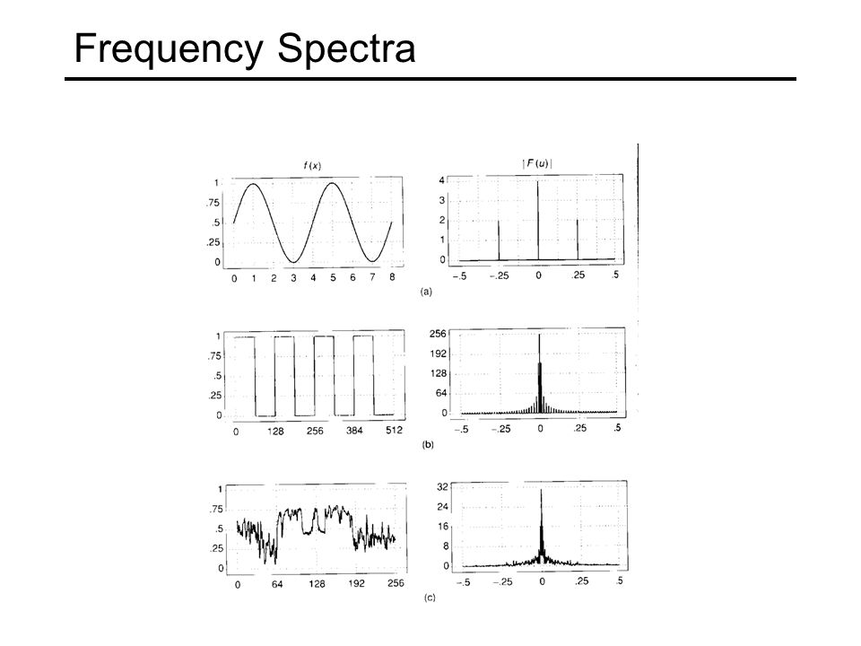
Frequency Spectra Usually, frequency is more interesting than the phase

13
= + = Frequency Spectra

14
= + =

15
= + =

16
= + =

17
= + =

18
=

20
Extension to 2D in Matlab, check out: imagesc(log(abs(fftshift(fft2(im)))));
))));")
21
Man-made Scene

22
Can change spectrum, then reconstruct

23
Low and High Pass filtering

24
The Convolution Theorem The greatest thing since sliced (banana) bread! The Fourier transform of the convolution of two functions is the product of their Fourier transforms The inverse Fourier transform of the product of two Fourier transforms is the convolution of the two inverse Fourier transforms Convolution in spatial domain is equivalent to multiplication in frequency domain!

25
2D convolution theorem example * f(x,y)f(x,y) h(x,y)h(x,y) g(x,y)g(x,y) |F(s x,s y )| |H(s x,s y )| |G(s x,s y )|
f(x,y) h(x,y)h(x,y) g(x,y)g(x,y) |F(s x,s y )| |H(s x,s y )| |G(s x,s y )|")
26
Fourier Transform pairs

27
Low-pass, Band-pass, High-pass filters low-pass: High-pass / band-pass:

28
Edges in images

29
What does blurring take away? original

30
What does blurring take away? smoothed (5x5 Gaussian)
")
31
High-Pass filter smoothed – original

32
Band-pass filtering Laplacian Pyramid (subband images) Created from Gaussian pyramid by subtraction Gaussian Pyramid (low-pass images)
 Created from Gaussian pyramid by subtraction Gaussian Pyramid (low-pass images)")
33
Laplacian Pyramid How can we reconstruct (collapse) this pyramid into the original image? Need this! Original image

34
Why Laplacian? Laplacian of Gaussian Gaussian delta function

35
Unsharp Masking - = = +

36
Image gradient The gradient of an image: The gradient points in the direction of most rapid change in intensity The gradient direction is given by: how does this relate to the direction of the edge? The edge strength is given by the gradient magnitude

37
Effects of noise Consider a single row or column of the image Plotting intensity as a function of position gives a signal Where is the edge? How to compute a derivative?

38
Where is the edge? Solution: smooth first Look for peaks in

39
Derivative theorem of convolution This saves us one operation:

40
Laplacian of Gaussian Consider Laplacian of Gaussian operator Where is the edge? Zero-crossings of bottom graph

41
2D edge detection filters is the Laplacian operator: Laplacian of Gaussian Gaussianderivative of Gaussian

42
Try this in MATLAB g = fspecial('gaussian',15,2); imagesc(g); colormap(gray); surfl(g) gclown = conv2(clown,g,'same'); imagesc(conv2(clown,[-1 1],'same')); imagesc(conv2(gclown,[-1 1],'same')); dx = conv2(g,[-1 1],'same'); imagesc(conv2(clown,dx,'same')); lg = fspecial('log',15,2); lclown = conv2(clown,lg,'same'); imagesc(lclown) imagesc(clown +.2*lclown)
![Try this in MATLAB g = fspecial( gaussian ,15,2); imagesc(g); colormap(gray); surfl(g) gclown = conv2(clown,g, same ); imagesc(conv2(clown,[-1 1], same )); imagesc(conv2(gclown,[-1 1], same )); dx = conv2(g,[-1 1], same ); imagesc(conv2(clown,dx, same )); lg = fspecial( log ,15,2); lclown = conv2(clown,lg, same ); imagesc(lclown) imagesc(clown +.2*lclown)](http://images.slideplayer.com/26/8684067/slides/slide_42.jpg "Try this in MATLAB g = fspecial( gaussian ,15,2); imagesc(g); colormap(gray); surfl(g) gclown = conv2(clown,g, same ); imagesc(conv2(clown,[-1 1], same )); imagesc(conv2(gclown,[-1 1], same )); dx = conv2(g,[-1 1], same ); imagesc(conv2(clown,dx, same )); lg = fspecial( log ,15,2); lclown = conv2(clown,lg, same ); imagesc(lclown) imagesc(clown +.2*lclown)")
43
Campbell-Robson contrast sensitivity curve

44
Depends on Color R GB

45
Lossy Image Compression (JPEG) Block-based Discrete Cosine Transform (DCT)
 Block-based Discrete Cosine Transform (DCT)")
46
Using DCT in JPEG The first coefficient B(0,0) is the DC component, the average intensity The top-left coeffs represent low frequencies, the bottom right – high frequencies
 is the DC component, the average intensity The top-left coeffs represent low frequencies, the bottom right – high frequencies")
47
Image compression using DCT DCT enables image compression by concentrating most image information in the low frequencies Loose unimportant image info (high frequencies) by cutting B(u,v) at bottom right The decoder computes the inverse DCT – IDCT Quantization Table 3 5 7 9 11 13 15 17 5 7 9 11 13 15 17 19 7 9 11 13 15 17 19 21 9 11 13 15 17 19 21 23 11 13 15 17 19 21 23 25 13 15 17 19 21 23 25 27 15 17 19 21 23 25 27 29 17 19 21 23 25 27 29 31
 by cutting B(u,v) at bottom right The decoder computes the inverse DCT – IDCT Quantization Table")
48
Block size in JPEG Block size small block –faster –correlation exists between neighboring pixels large block –better compression in smooth regions It’s 8x8 in standard JPEG

49
JPEG compression comparison 89k12k

50
Morphological Operation What if your images are binary masks? Binary image processing is a well-studied field, based on set theory, called Mathematical Morphology

51
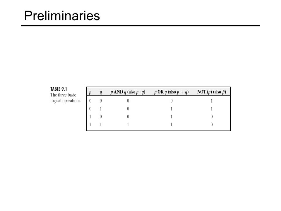
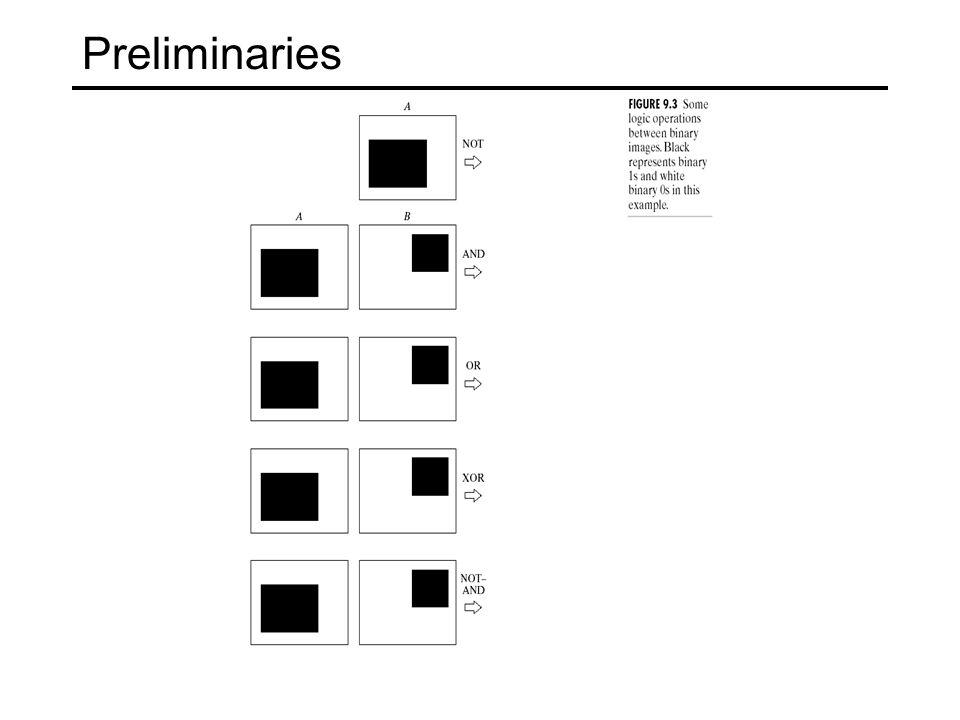
Preliminaries

54
Basic Concepts in Set Theory A is a set in, a=(a 1,a 2 ) an element of A, a A If not, then a A : null (empty) set Typical set specification: C={w|w=-d, for d D} A subset of B: A B Union of A and B: C=A B Intersection of A and B: D=A B Disjoint sets: A B= Complement of A: Difference of A and B: A-B={w|w A, w B}=
 an element of A, a A If not, then a A : null (empty) set Typical set specification: C={w|w=-d, for d D} A subset of B: A B Union of A and B: C=A B Intersection of A and B: D=A B Disjoint sets: A B= Complement of A: Difference of A and B: A-B={w|w A, w B}=")
55
Preliminaries

56
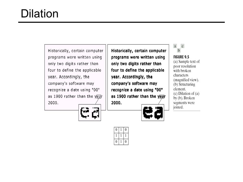
Dilation and Erosion Two basic operations: A is the image, B is the “structural element”, a mask akin to a kernel in convolution Dilation : (all shifts of B that have a non-empty overlap with A) Erosion : (all shifts of B that are fully contained within A)
 Erosion : (all shifts of B that are fully contained within A)")
57
Dilation

59
Erosion

60
Original image Eroded image

61
Erosion Eroded once Eroded twice

62
Opening and Closing Opening : smoothes the contour of an object, breaks narrow isthmuses, and eliminates thin protrusions Closing : smooth sections of contours but, as opposed to opning, it generally fuses narrow breaks and long thin gulfs, eliminates small holes, and fills gaps in the contour Prove to yourself that they are not the same thing. Play around with bwmorph in Matlab.

63
OPENING: The original image eroded twice and dilated twice (opened). Most noise is removed Opening and Closing CLOSING: The original image dilated and then eroded. Most holes are filled.

64
Opening and Closing

65
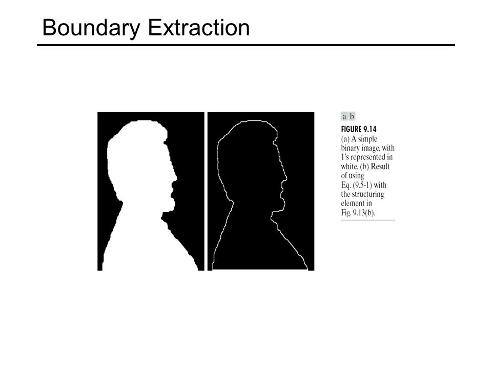
Boundary Extraction

Similar presentations


>")


![Reminder Fourier Basis: t [0,1] nZnZ Fourier Series: Fourier Coefficient:](/16/4936498/big_thumb.jpg "Reminder Fourier Basis: t [0,1] nZnZ Fourier Series: Fourier Coefficient:>")


