Download presentation
Presentation is loading. Please wait.

1
Where are the radars located? What is the radar coverage?
Radar Systems Where are the radars located? What is the radar coverage? What are some of the characteristics that differentiate between radar systems? Radar Scan strategies? Radar products?

2
Radar History – in Brief
Radar Radio Detection And Ranging In 1887, a physicist named Heinrich Hertz began experimenting with radio waves in his laboratory in Germany. Sir Robert Alexander Watson-Watt ( ) Watson-Watt was the Scottish physicist who developed the radar locating of aircraft in England. Radar was patented (British patent) in April, 1935. Doppler RADAR is named after Christian Andreas Doppler, an Austrian physicist who first described in 1842, how the observed frequency of light and sound waves was affected by the relative motion of the source and the detector. This phenomenon became known as the Doppler effect. Weather radar. started in 1943 as a Canadian Army project in Ottawa
 Watson-Watt was the Scottish physicist who developed the radar locating of aircraft in England. Radar was patented (British patent) in April, Doppler RADAR is named after Christian Andreas Doppler, an Austrian physicist who first described in 1842, how the observed frequency of light and sound waves was affected by the relative motion of the source and the detector. This phenomenon became known as the Doppler effect. Weather radar. started in 1943 as a Canadian Army project in Ottawa.")
4
North American Radar Coverage

5
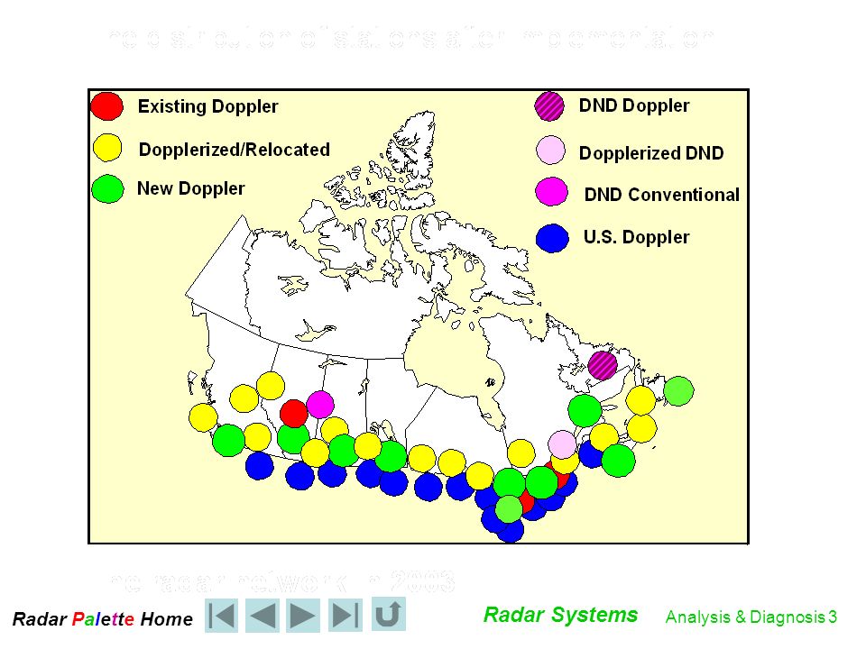
Canadian Radar Coverage – Canadian Composite
For the masses….

6
Nominal Radar Coverage with 256 km range
However, in winter …

7
Effective Radar Coverage with 2 km echo tops
Large blind swaths across the country ♫ I’m dreaming of gap-filling X-band network … Even here on the 401

8
Pacific Network

9
Prairie Network

10
Ontario Network

11
Quebec Network

12
Atlantic Network

13
Radar Data in Ontario

14
NWS Radar Composite Meteorologists without Borders

15
Antenna Scan Strategies
Conventional: 24 PPI scans top down 6 RPM 24.6 to 0.3 degrees (0.1 in winter) 5 minutes to complete 10 seconds per elevation angle, 6 per minute Doppler: 3 scan angles bottom up ? much slower (0.85 RPM) since more sample points are collected for the Doppler processing fills much of remaining 5 minutes 10 minute cycle
 5 minutes to complete. 10 seconds per elevation angle, 6 per minute. Doppler: 3 scan angles. bottom up much slower (0.85 RPM) since more sample points are collected for the Doppler processing. fills much of remaining 5 minutes. 10 minute cycle.")
16
Some basic radar products CAPPI vs. PRECIP
Uses conventional reflectivity scans 1 km AGL out to 100 km, then rides up the lowest PPI angle (~0.1° winter & 0.3 ° summer) out to 256 km Precipitation is relatively high above ground and can grow considerably between 1 km AGL and the surface PRECIP Uses long range doppler reflectivity scan within 125 km of radar, including ground clutter removal Uses lowest PPI conventional reflectivity scan beyond 125 km of radar Doppler reflectivity not quite as sensitive to weak echoes Best product for seeing precipitation close to ground Therefore, Precipitation Accums (PA) from PRECIP product should be better than from CAPPI, as long as ground doesn’t absorb too much beam power
 out to 256 km. Precipitation is relatively high above ground and can grow considerably between 1 km AGL and the surface. PRECIP. Uses long range doppler reflectivity scan within 125 km of radar, including ground clutter removal. Uses lowest PPI conventional reflectivity scan beyond 125 km of radar. Doppler reflectivity not quite as sensitive to weak echoes. Best product for seeing precipitation close to ground. Therefore, Precipitation Accums (PA) from PRECIP product should be better than from CAPPI, as long as ground doesn’t absorb too much beam power.")
17
Some basic radar products
CAPPI 1.0 km vs. PRECIP product 2 10 18 CAPPI 1.0 PRECIP beam height (km) 0.0 0 2.0 0 25.0 0 Doppler reflectivity Conventional reflectivity range (km)
 Doppler reflectivity Conventional reflectivity. range (km)")
18
PRECIP product example
Boundary between doppler & conventional reflectivity scans

19
The smaller the beamwidth, better the gain
Gain vs Beamwidth The smaller the beamwidth, better the gain Improved gain means higher signal strength for distant objects or small targets e.g. light precipitation may be detected at greater distances

20
Weather Radar Bands The more common weather radar wavelengths and letter designations are:

21
Pulse Repetition Frequency (PRF)
The pulse repetition frequency (PRF) is the number of pulses emitted by the radar per second (pps) A pulse travelling to a target at range rmax and back will cover a distance 2rmax The pulse will make it back to the radar before the next pulse is emitted if: 2rmax=c/PRF
 is the number of pulses emitted by the radar per second (pps) A pulse travelling to a target at range rmax and back will cover a distance 2rmax. The pulse will make it back to the radar before the next pulse is emitted if: 2rmax=c/PRF.")
22
rmax=c/2PRF PRF and radar range
Or…. rmax=c/2PRF Thus, the higher the PRF, the lower the effective range (ignoring second-trip echos from objects located beyond rmax) The lower the PRF, the higher the range.
 The lower the PRF, the higher the range.")
23
Rmax vs PRF

24
Rmax in selected modes The Clear Air PRF is 50 allowing greater range.

25
CONVENTIONAL RADAR DISPLAYS
PPI CAPPI FOUR CAPPI MAX R ECHO TOP SEVERE WEATHER CROSS SECTION STYLE: DIAMETER CROSS SECTION ARBITRARY CROSS SECTION

26
PPI Elevations and Angles
The CAPPI level is set from the KING95 parameter file, and may be any value between 0.0 and 20.0 km. The 1.5 km CAPPI in summer and 1.0 km in winter have proved to be the most useful displays for operational use and public consumption. These are about the lowest altitudes that can be produced without excessive ground effects and the data closely approximate the precipitation reaching ground level at the time. The lower level CAPPI for winter aids in showing any lighter and lower altitude snowfall activity prevalent in many snow flurry and snow streamer situations. A request for a 0.0 km CAPPI results in the 0.3° PPI surface. The CAPPI product provides a credible horizontal presentation of echoes, but at times will require some interpretation. Notably, it will be seen from Figure 1., that the very low altitude CAPPI surfaces, i.e km, are in reality saucer shaped, with the surface rising beyond about 120 km due to the earth's curvature. The maximum Z value encountered on the CAPPI surface is displayed on the text line above the range/pixel scale with the following syntax: Z: AAA, RRR, , ZZ where, AAA = azimuth in degrees RRR = range in km ZZ = maximum Z value in dBZe In this product, the Colour Table displays the echo intensity values in both dBZ (dBZi) and precipitation rate. The threshold scale is selected by the KING95 parameter file.
 and precipitation rate. The threshold scale is selected by the KING95 parameter file.")
27
Radar beam height vs. range
Height of radar beam in normal atmospheric conditions 2 10 18 Cone of silence 0.0 0 2.0 0 25.0 0 beam height (km) 1.00 beam Beam widens with range range (km) Overshoots low tops
 1.00 beam. Beam widens with range. range (km) Overshoots low tops.")
28
PPI Display - 0.3 Degree Angle

29
PPI and CAPPI 4.0 km CAPPI The CAPPI level is set from the KING95 parameter file, and may be any value between 0.0 and 20.0 km. The 1.5 km CAPPI in summer and 1.0 km in winter have proved to be the most useful displays for operational use and public consumption. These are about the lowest altitudes that can be produced without excessive ground effects and the data closely approximate the precipitation reaching ground level at the time. The lower level CAPPI for winter aids in showing any lighter and lower altitude snowfall activity prevalent in many snow flurry and snow streamer situations. A request for a 0.0 km CAPPI results in the 0.3° PPI surface. The CAPPI product provides a credible horizontal presentation of echoes, but at times will require some interpretation. Notably, it will be seen from Figure 1., that the very low altitude CAPPI surfaces, i.e km, are in reality saucer shaped, with the surface rising beyond about 120 km due to the earth's curvature. The maximum Z value encountered on the CAPPI surface is displayed on the text line above the range/pixel scale with the following syntax: Z: AAA, RRR, , ZZ where, AAA = azimuth in degrees RRR = range in km ZZ = maximum Z value in dBZe In this product, the Colour Table displays the echo intensity values in both dBZ (dBZi) and precipitation rate. The threshold scale is selected by the KING95 parameter file. 0.3 Degree PPI 1.5km CAPPI 0.3 Degree PPI
 and precipitation rate. The threshold scale is selected by the KING95 parameter file. 0.3 Degree PPI. 1.5km CAPPI. 0.3 Degree PPI.")
30
CAPPI The Constant Altitude Plan Position Indicator (CAPPI) display was devised to present the echo data in a PPI format but on a pseudo-horizontal surface for any altitude. This product has a simpler dynamic analysis potential, and provides the user a better visualization of the horizontal distribution of echoes. If the antenna is rotated uniformly in azimuth and lowered in elevation by steps after each revolution, by selecting an appropriate range interval for each elevation, a series of annular rings can be swept out centred on any selected altitude. Data from this set of annular rings can then be meshed together to synthesize a near-horizontal surface. Figure 1 shows the antenna beam axes locations for the construction of CAPPI displays at 2 different altitudes, 1.5 km and 4.0 km. Note, to avoid smoothing of important characteristics, the near-horizontal surface is not interpolated between beam axes, but instead snaps to use the closest beam axis. The figure accentuates the layer irregularity due to the difference in scale of the vertical and horizontal axes, but these discontinuities are nevertheless present and explain the occasional aberrations which may occur with certain echo patterns. Attempting to reduce these discontinuities by improving horizontal resolution with more elevations, unfortunately also increases the total scanning cycle time to beyond acceptable limits. Then finally from the newly meshed radial array, the Cartesian (pixel) array is extracted using the co-ordinate Lookup Table.
 display was devised to present the echo data in a PPI format but on a pseudo-horizontal surface for any altitude. This product has a simpler dynamic analysis potential, and provides the user a better visualization of the horizontal distribution of echoes. If the antenna is rotated uniformly in azimuth and lowered in elevation by steps after each revolution, by selecting an appropriate range interval for each elevation, a series of annular rings can be swept out centred on any selected altitude. Data from this set of annular rings can then be meshed together to synthesize a near-horizontal surface. Figure 1 shows the antenna beam axes locations for the construction of CAPPI displays at 2 different altitudes, 1.5 km and 4.0 km. Note, to avoid smoothing of important characteristics, the near-horizontal surface is not interpolated between beam axes, but instead snaps to use the closest beam axis. The figure accentuates the layer irregularity due to the difference in scale of the vertical and horizontal axes, but these discontinuities are nevertheless present and explain the occasional aberrations which may occur with certain echo patterns. Attempting to reduce these discontinuities by improving horizontal resolution with more elevations, unfortunately also increases the total scanning cycle time to beyond acceptable limits. Then finally from the newly meshed radial array, the Cartesian (pixel) array is extracted using the co-ordinate Lookup Table.")
31
Cross-sections - CAPPI - Echo Top

32
MAXR Data Display

33
Severe Weather Display
Radar is a tool that requires careful and knowledgeable interpretation.

Similar presentations


 Atlas (1989)>")


 -12 dBZ. Echoes in clear air from insects Common is summer. Watch for echoes to expand area as sun sets and insects.>")

 Eric WATTRELOT & Jean-François MAHFOUF (Météo-France/CNRM/GMAP)>")


 MSC Radar Course Paul Ford Lead Instructor MOIP Dartmouth.>")
 Your Organization (Line #2) Basics of Radar Joe Hoatam Josh Merritt Aaron Nielsen.>")


