Download presentation
Presentation is loading. Please wait.

2
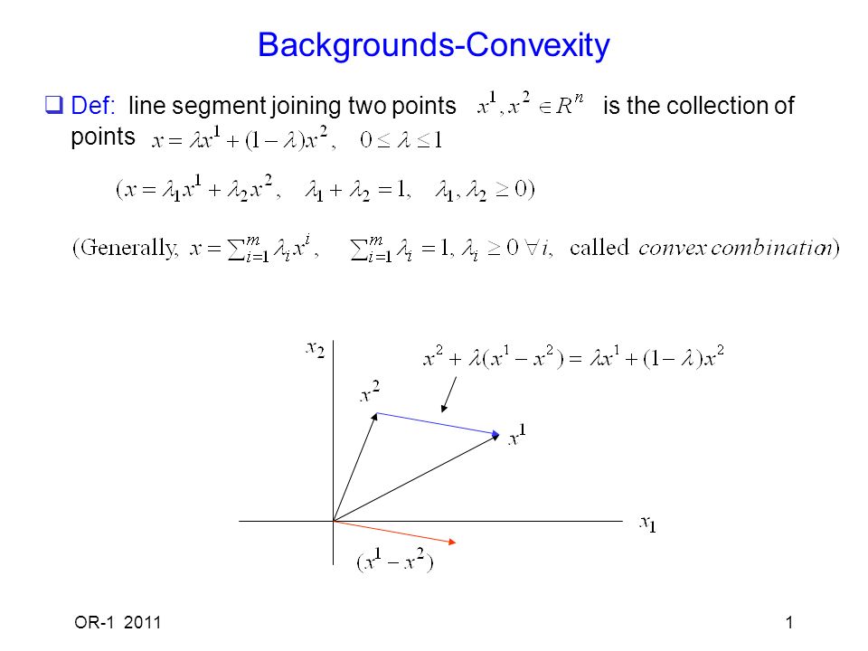
OR-1 20111 Backgrounds-Convexity Def: line segment joining two points is the collection of points

3
OR-1 20112 Def: is called convex set iff whenever Convex sets Nonconvex set

4
OR-1 20113 Def: The convex hull of a set S is the set of all points that are convex combinations of points in S, i.e. conv(S)={x: x = i = 1 k i x i, k 1, x 1,…, x k S, 1,..., k 0, i = 1 k i = 1} Picture: 1 x + 2 y + 3 z, i 0, i = 1 3 i = 1 1 x + 2 y + 3 z = ( 1 + 2 ){ 1 /( 1 + 2 )x + 2 /( 1 + 2 )y} + 3 z (assuming 1 + 2 0) x y z
={x: x = i = 1 k i x i, k 1, x 1,…, x k S, 1,..., k 0, i = 1 k i = 1} Picture: 1 x + 2 y + 3 z, i 0, i = 1 3 i = 1 1 x + 2 y + 3 z = ( ){ 1 /( )x + 2 /( )y} + 3 z (assuming 0) x y z.")
5
OR-1 20114 Proposition: Let be a convex set and for, define Then is a convex set. Pf) If k = 0, kC is convex. Suppose For any x, y kC, Hence the property of convexity of a set is preserved under scalar multiplication. Consider other operations that preserve convexity.
 If k = 0, kC is convex. Suppose For any x, y kC, Hence the property of convexity of a set is preserved under scalar multiplication. Consider other operations that preserve convexity..")
6
OR-1 20115 Convex function Def: Function is called a convex function if for all x 1 and x 2, f satisfies Also called strictly convex function if

7
Meaning: The line segment joining (x 1, f(x 1 )) and (x 2, f(x 2 )) is above or on the locus of points of function values. OR-1 20116

8
7 Def: f: R n R. Define epigraph of f as epi(f) = { (x, ) R n+1 : f(x) } Equivalent definition: f: R n R is a convex function if and only if epi(f) is a convex set. Def: f is a concave function if –f is a convex function. Def: x C is an extreme point of a convex set C if x cannot be expressed as y + (1- )z, 0 < < 1 for distinct y, z C ( x y, z ) (equivalently, x does not lie on any line segment that joins two other points in the set C.) : extreme points
 = { (x, ) R n+1 : f(x) } Equivalent definition: f: R n R is a convex function if and only if epi(f) is a convex set. Def: f is a concave function if –f is a convex function. Def: x C is an extreme point of a convex set C if x cannot be expressed as y + (1- )z, 0 < < 1 for distinct y, z C ( x y, z ) (equivalently, x does not lie on any line segment that joins two other points in the set C.) : extreme points.")
9
OR-1 20118 Review-Linear Algebra inner product of two column vectors x, y R n : x’y = i = 1 n x i y i If x’y = 0, x, y 0, then x, y are said to be orthogonal. In 3-D, the angle between the two vectors is 90 degrees. ( Vectors are column vectors unless specified otherwise. But, our text does not differentiate it.)
.")
10
OR-1 20119 Submatrices multiplication

11
OR-1 201110 submatrices multiplications which will be frequently used.

12
OR-1 201111 Def: is said to be linearly dependent if , not all equal to 0, such that ( i.e., there exists a vector in which can be expressed as a linear combination of the other vectors. ) Def: linearly independent if not linearly dependent. In other words, (i.e., none of the vectors in can be expressed as a linear combination of the remaining vectors.) Def: Rank of a set of vectors : maximum number of linearly independent vectors in the set. Def: Basis for a set of vectors : collection of linearly independent vectors from the set such that every vector in the set can be expressed as a linear combination of them. (maximal linearly independent subset, minimal generator of the set)
 Def: linearly independent if not linearly dependent. In other words, (i.e., none of the vectors in can be expressed as a linear combination of the remaining vectors.) Def: Rank of a set of vectors : maximum number of linearly independent vectors in the set. Def: Basis for a set of vectors : collection of linearly independent vectors from the set such that every vector in the set can be expressed as a linear combination of them. (maximal linearly independent subset, minimal generator of the set).")
13
OR-1 201112 Thm) r linearly independent vectors form a basis if and only if the set has rank r. Def: row rank of a matrix : rank of its set of row vectors column rank of a matrix : rank of its set of column vectors Thm) for a matrix A, row rank = column rank Def : nonsingular matrix : rank = number of rows = number of columns. Otherwise, called singular Thm) If A is nonsingular, then unique inverse exists.
 for a matrix A, row rank = column rank Def : nonsingular matrix : rank = number of rows = number of columns. Otherwise, called singular Thm) If A is nonsingular, then unique inverse exists..")
14
OR-1 201113 Simutaneous Linear Equations Thm: Ax = b has at least one solution iff rank(A) = rank( [A, b] ) Pf) ) rank( [A, b] ) rank(A). Suppose rank( [A, b] ) > rank(A). Then b is lin. ind. of the column vectors of A, i,e., b can’t be expressed as a linear combination of columns of A. Hence Ax = b does not have a solution. ) There exists a basis in columns of A which generates b. So Ax = b has a solution. Suppose A: m n, rank(A) = rank [A, b] = r. Then Ax = b has a unique solution if r = n. Pf) Let y, z be any two solutions of Ax = b. Then Ay = Az = b, or Ay – Az = A(y-z) = 0. A(y-z) = j=1 n A j (y j – z j ) = 0. Since column vectors of A are linearly independent, we have y j – z j = 0 for all j. Hence y = z. (Note that m may be greater than n.)
![OR Simutaneous Linear Equations Thm: Ax = b has at least one solution iff rank(A) = rank( [A, b] ) Pf) ) rank( [A, b] ) rank(A).](http://images.slideplayer.com/26/8451688/slides/slide_14.jpg "Suppose rank( [A, b] ) > rank(A). Then b is lin. ind. of the column vectors of A, i,e., b can’t be expressed as a linear combination of columns of A. Hence Ax = b does not have a solution. ) There exists a basis in columns of A which generates b. So Ax = b has a solution. Suppose A: m n, rank(A) = rank [A, b] = r. Then Ax = b has a unique solution if r = n. Pf) Let y, z be any two solutions of Ax = b. Then Ay = Az = b, or Ay – Az = A(y-z) = 0. A(y-z) = j=1 n A j (y j – z j ) = 0. Since column vectors of A are linearly independent, we have y j – z j = 0 for all j. Hence y = z. (Note that m may be greater than n.).")
15
OR-1 201114

16
OR-1 201115 Operations that do not change the solution set of the linear equations (Elementary row operations) Change the position of the equations Multiply a nonzero scalar k to both sides of an equation Multiply a scalar k to an equation and add it to another equation Hence X = Y. Solution sets are same. The operations can be performed only on the coefficient matrix [A, b], for Ax = b.

17
OR-1 201116 Solving systems of linear equations (Gauss-Jordan Elimination, 변수의 치환 ) (will be used in the simplex method to solve LP problems)
 (will be used in the simplex method to solve LP problems)")
18
OR-1 201117 Infinitely many solutions

19
OR-1 201118

20
OR-1 201119

21
OR-1 201120 Elementary row operations are equivalent to premultiplying a nonsingular square matrix to both sides of the equations Ax = b

22
OR-1 201121

23
OR-1 201122

24
OR-1 201123 So if we multiply all elementary row operation matrices, we get the matrix having the information about the elementary row operations we performed

25
OR-1 201124 Finding inverse of a nonsingular matrix A. Perform elementary row operations (premultiply elementary row operation matrices) to make [A : I ] to [ I : B ] Let the product of the elementary row operations matrices be C. Then C [ A : I ] = [ CA : C ] = [ I : B] Hence CA = I C = A -1 and B = A -1.
 to make [A : I ] to [ I : B ] Let the product of the elementary row operations matrices be C. Then C [ A : I ] = [ CA : C ] = [ I : B] Hence CA = I C = A -1 and B = A -1..")
26
OR-1 201125

Similar presentations