Download presentation
Presentation is loading. Please wait.

1
Sensitivity experiments with the Runge Kutta time integration scheme Lucio TORRISI CNMCA – Pratica di Mare (Rome) l.torrisi@meteoam.it
")
2
Introduction A new dynamical core has been developed in LM (Forstner and Doms, 2004). It is based on a TVD variant of 3rd-order Runge Kutta time integration scheme (RK) using a 5th-order spatial discretization of advection. The RK core should be more accurate than the standard Leap-Frog/2nd-order advection scheme (LF) and it will be used for very detailed short range forecasts. RK core needs to be tested and evaluated, before it can be operationally implemented.
 using a 5th-order spatial discretization of advection. The RK core should be more accurate than the standard Leap-Frog/2nd-order advection scheme (LF) and it will be used for very detailed short range forecasts. RK core needs to be tested and evaluated, before it can be operationally implemented..")
3
Overview LM configuration and verification method. RK compared to LF. RK sensitivity to the: - integration time step (72s, 48s); - interval between two calls of some parameterizations (convection, turbulence); - turbulence parameterization scheme (diagnostic and prognostic TKE); - domain size; - moisture variables advection scheme (eulerian, semi-lagrangian); - moisture variables transport formulation. Summary and conclusion.
; - interval between two calls of some parameterizations (convection, turbulence); - turbulence parameterization scheme (diagnostic and prognostic TKE); - domain size; - moisture variables advection scheme (eulerian, semi-lagrangian); - moisture variables transport formulation. Summary and conclusion..")
5
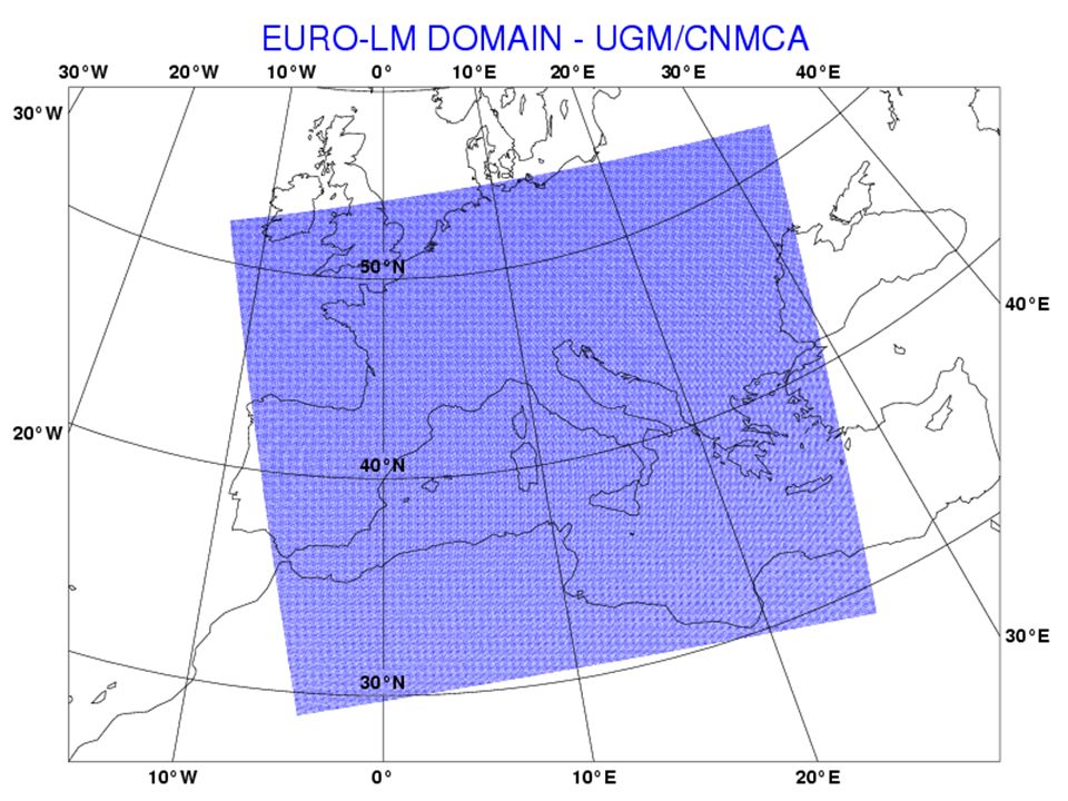
EXPERIMENTAL RUN ON FUJITSU (ECMWF) LM CONFIGURATION (version 2.10) Domain size465 x 385 (EuroLM) Grid spacing0.0625 (7 km) Number of layers35 Time step72 sec Forecast range24 hrs Initial time of model run00 UTC Lateral boundary conditions and initial stateOp. IFS (preproc. with CNMCA-IFS2LM) L.B.C. update frequency3 hrs OrographyFiltered (eps = 0.1) Prognostic precipitationOn Rayleigh damping schemeRelaxation to LM filtered fields Interval between two calls of turbulence1 time step Turbulence parameterizationPrognostic TKE R.damping: filter iteration number10 R. damping: filter length1 LM configuration (v. 3.16+) Domain size234 x 272 Grid spacing0.0625 (7 km) Number of layers35 Time step and integration scheme40 sec, 3 timelevel split-explicit Forecast range48 hrs Initial time of model run00/12 UTC Lateral boundary conditionsGME L.B.C. update frequency1 hrs Initial stateGME InitializationD. F. External analysisNone StatusOperational HardwareIBM SP3 (Bologna) N° of processors used64
 L.B.C. update frequency3 hrs OrographyFiltered (eps = 0.1) Prognostic precipitationOn Rayleigh damping schemeRelaxation to LM filtered fields Interval between two calls of turbulence1 time step Turbulence parameterizationPrognostic TKE R.damping: filter iteration number10 R. damping: filter length1 LM configuration (v ) Domain size234 x 272 Grid spacing (7 km) Number of layers35 Time step and integration scheme40 sec, 3 timelevel split-explicit Forecast range48 hrs Initial time of model run00/12 UTC Lateral boundary conditionsGME L.B.C. update frequency1 hrs Initial stateGME InitializationD. F. External analysisNone StatusOperational HardwareIBM SP3 (Bologna) N° of processors used64.")
6
Objective verification method Statistical verification through comparison of LM forecasts with lowland station observations in the period 24 – 28 March 2005 (5 runs). Nearest grid point is used as LM forecast. Only land stations with h<700m and height mismatch with model topography less than 100m were used. About 3500 fc-obs pairs were used to calculate the mean error and RMSE of the surface variables forecast. They are enough to make statistical comparisons between different configurations of LM.

8
LF (40s) compared to RK (72s)
 compared to RK (72s)")
14
RK performs worse than LF for MSLP forecasts due to a large bias (also small differences in other surface variables and wind vector). RK has a slightly smaller upper level temperature RMSE. RK and LF use different time steps that determine a different time interval between two calls of physics. One experiment to find out the cause of the MSLP deficiency in RK could be to decrease the time step from 72s to 40s (time step for LF), in order to have the same parameterizations calling frequency for LF and RK.
, in order to have the same parameterizations calling frequency for LF and RK..")
15
RK (40s) compared to RK (72s)
 compared to RK (72s)")
16
RK with 40s time step has a slightly smaller MSLP bias than RK with 72s time step at T+18h and T+24h. This result seems to be due to the higher accuracy associated with the smaller time step. To totally exclude the influence of the interval between two calls of parameterization schemes, some experiments are useful. One experiment is to decrease the convection calling frequency nincconv from 10 to 5. Another experiment is to increase the interval between two calls of the prognostic TKE turbulence scheme ninctura from 1 to 2 (every two time steps instead of every time step).
..")
17
RK (40s) with ninctura = 1, 2 or with nincconv = 10, 5
 with ninctura = 1, 2 or with nincconv = 10, 5")
18
RK is not significantly sensitive to the calling frequency of the convection and prognostic TKE turbulence scheme. What is the behaviour of the diagnostic TKE turbulence scheme compared to the prognostic one? RK (40s) with ninctura = 1, 2 or with nincconv = 10, 5
 with ninctura = 1, 2 or with nincconv = 10, 5.")
19
RK with new and old turbulence

21
RK with the old turbulence scheme seems to perform better (smaller bias and standard deviation) than RK with the prognostic TKE turbulence parameterization. The improvement in the MSLP bias is related to the low level positive temperature bias of RK with old turbulence. The prognostic TKE turbulence parameterization seems to be one of the likely candidate to justify the MSLP forecast deficiency in RK. However, a large bias is still present! How does RK with old turbulence perform compared to the LF? RK with new and old turbulence

22
LF and RK with old turbulence

24
Using the old turbulence scheme the large MSLP bias difference between RK and LF is slightly reduced. A positive MSLP bias (except for T+12h) is present in RK, but a slightly smaller standard deviation than in LF is also found. Some tuning of the RK+physics core is necessary to reduce the large bias in MSLP forecast (cold bias in upper levels), but the slight improvement in the standard deviation seems to be an indication of the higher-order accuracy of the RK compared to the LF. LF and RK with old turbulence
 is present in RK, but a slightly smaller standard deviation than in LF is also found. Some tuning of the RK+physics core is necessary to reduce the large bias in MSLP forecast (cold bias in upper levels), but the slight improvement in the standard deviation seems to be an indication of the higher-order accuracy of the RK compared to the LF. LF and RK with old turbulence.")
25
RK with different domain sizes

26
The enlargement of the domain size seems to have a negative impact (larger RMSE for forecast times greater than T+6h) on the MSLP forecast. A similar result was obtained for a longer period using the LF (Torrisi, 2005). The increase of the standard deviation could be related to the improvement of the intrinsic variability of the model associated with the enlargement of the domain (BC are slightly affecting the forecast). RK with different domain sizes
. The increase of the standard deviation could be related to the improvement of the intrinsic variability of the model associated with the enlargement of the domain (BC are slightly affecting the forecast). RK with different domain sizes.")
27
RK with Eulerian and SL moisture variables advection

29
The SL moisture advection scheme does not show any significant difference in MSLP forecast compared to the Eulerian one (slightly larger standard deviation after T+18h balanced by a slightly smaller bias), but it seems to have a slightly better skill for 6h accumulated precipitation. RK with Eulerian and SL moisture variables advection

30
RK with conservation form of moisture variables transport

32
The conservative form of the moisture variables transport has a larger MSLP bias than the default formulation. A slight improvement after T+18h is obtained switching on the prognostic advection of density. RK with conservation form of moisture variables transport

33
Summary and Conclusion The comparison of LF and RK schemes was performed for a 5 days period using the EuroLM configuration. Statistical verification results showed that RK performance for surface variables was slightly better than LF one. A large MSLP bias was typical of the RK runs. Some sensitivity studies were performed on RK to determine the cause of the MSLP forecast deficiency. RK did not show any sensitive to the calls of the prognostic TKE turbulence and convection schemes. An improvement in the MSLP forecast was obtained using the old turbulent scheme, but a larger bias was found again. The impact of the domain size and different moisture variables transport formulations was also evaluated. More work, especially investigations on the numerics- physics interaction, are needed to improve the RK core.

Similar presentations


 Research Applications Laboratory (RAL) and Developmental Testbed.>")


>")


>")
