1. IMF Prediction with Cosmic Rays THE BASIC IDEA: Find signatures in the cosmic ray flux that are predictive of the future behavior of the interplanetary magnetic field High-energy cosmic rays impacting Earth have passed through and interacted with the IMF within a region of size ~1 particle gyroradius – They should retain signatures related to the characteristics of the IMF Neutron monitors respond to ~10 GeV protons – These protons have a gyroradius ~0.04 AU, corresponding to a solar wind transit time of ~4 h Muon detectors respond to ~50 GeV protons – Gyroradius is ~0.2 AU, corresponding to a solar wind transit time of ~20 h The method can potentially fill in the gap between observations at L1 and observations of the Sun

2. IMF PREDICTION WITH COSMIC RAYS Based on Quasilinear Theory (QLT)

3. ENSEMBLE-AVERAGING DERIVATION OF THE BOLTZMANN EQUATION: START WITH THE VLASOV EQUATION The equation is relativistically correct

4. ENSEMBLE AVERAGE THE VLASOV EQUATION

5. SIMPLIFY THE ENSEMBLE-AVERAGED EQUATION WITH A TRICK For gyrotropic distributions, only ψ 1 matters!

6. SUBTRACT THE ENSEMBLE-AVERAGED EQUATION FROM THE ORIGINAL EQUATION … THEN LINEARIZE Why “Quasi”–Linear? 2 nd order terms are retained in the ensemble-averaged equation, but dropped in the equation for the fluctuations δf

7. AFTER LINEARIZING, IT’S EASY TO SOLVE FOR δf BY THE METHOD OF CHARACTERISTICS In effect, this integrates the fluctuating force backwards along the particle trajectory. “z” here is the mean Field direction, NOT GSE North This is like tomography, but using a helical “line of sight”

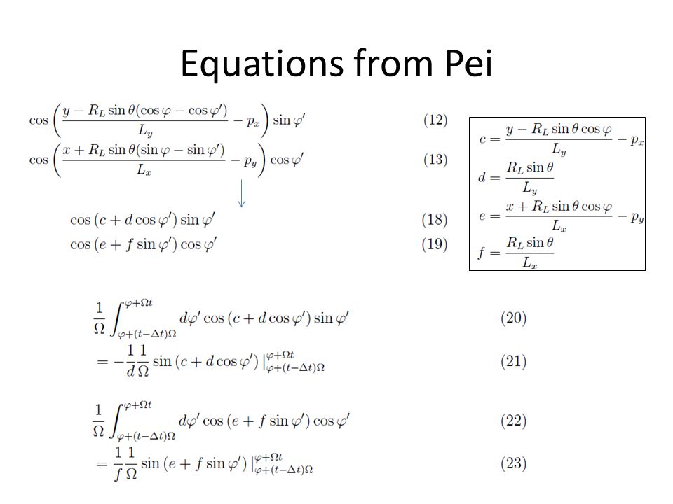
8. Equations from Pei

10. So, the integration of t is solved as

11. Spaceship Earth Spaceship Earth is a network of neutron monitors strategically deployed to provide precise, real-time, 3- dimensional measurements of the cosmic ray angular distribution: 11 Neutron Monitors on 4 continents Multi-national participation: – Bartol Research Institute, University of Delaware (U.S.A.) – IZMIRAN (Russia) – Polar Geophysical Inst. (Russia) – Inst. Solar-Terrestrial Physics (Russia) – Inst. Cosmophysical Research and Aeronomy (Russia) – Inst. Cosmophysical Research and Radio Wave Propagation (Russia) – Australian Antarctic Dvivision – Aurora College (Canada)

12. Data Pre-processing To select the intensity variation that would be sensitive to the IMF, we subtract isotropic component and 12 hour trailing-averaged anisotropy from observed NM intensity where f 0 and ξ are determined for each hour from the following best fit function

13. Data Pre-processing Observed intensity After subtract isotropic component And after subtract 1 st order anisotropic component Data during GLE is removed

14. Best-fit to the data fit this function to the cosmic ray flux and get 4 parameters A x, A y, p x, p y

15. estimation of dB * dB obs is calculated as the deviation from 12-hour tr-moving average of observed IMF in GSE coordinate. * dB exp is calculated from the model in IMF coordinate as

16. Conversion of coordinate IMF coordinate X imf is in X gse -Y gse plane Y imf is pointing north ward, and in Z imf -Z gse plane  X gse Y gse Z gse Z imf X imf Y imf  IMF

17. A : asymptotic viewing direction of particle calculated from particle trajectory code in gse coordinate then converted to imf coordinate Z imf X imf Y imf A IMF

18. GSE Lat -180 GSE Lat +180 Pitch angleGyro Phase Away Toward

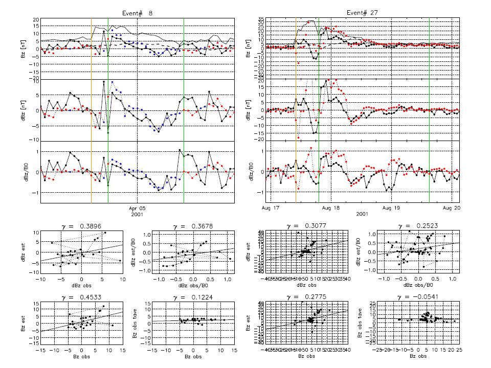
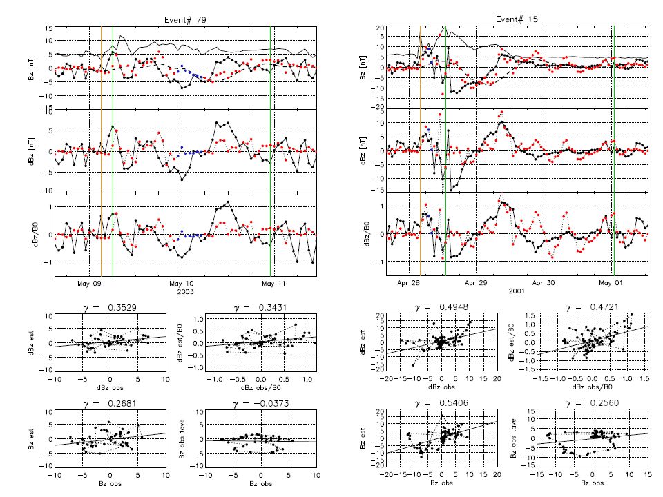
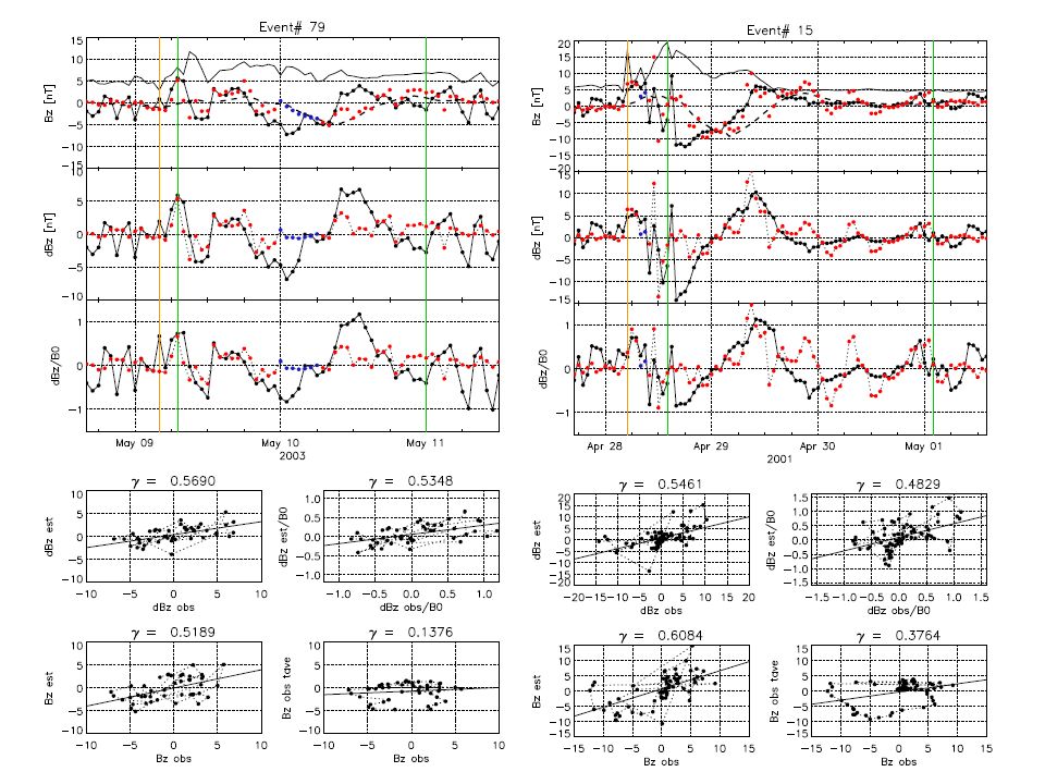
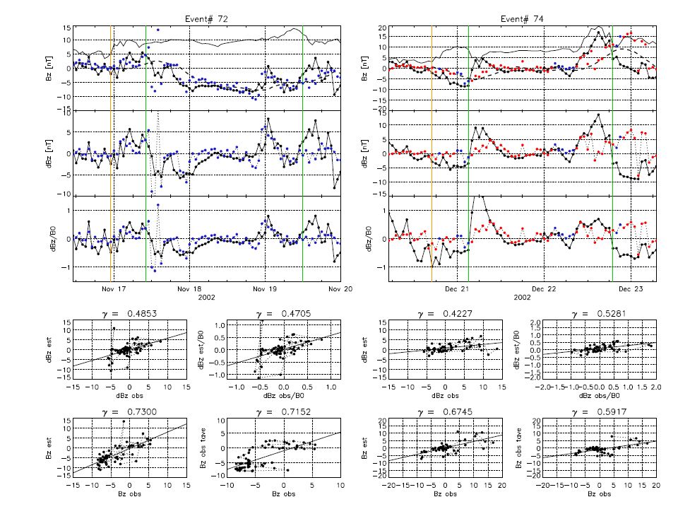
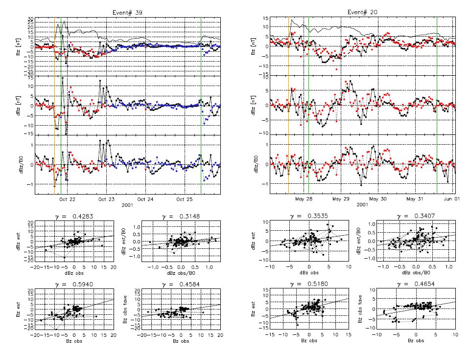
19. ICME Events Use ICME List from Richardson & Cane 2010, Solar Phys http://www.ssg.sr.unh.edu/mag/ace/ACEl ists/ICMEtable.html 161 ICMEs are listed from 2001 to 2006 Compare the IMF during the time from the IP Shock arrival time to the ICME end time Use hourly OMNI data (time corrected ACE or WIND) for the comparison of in-situ IMF data ICME Shock

20. ICME Shock dBz0.3896 dBz/Bt0.3678 Bz0.4533 Bz vs tave of Bz0.1224

24. dt=0 dt=1 dt=2

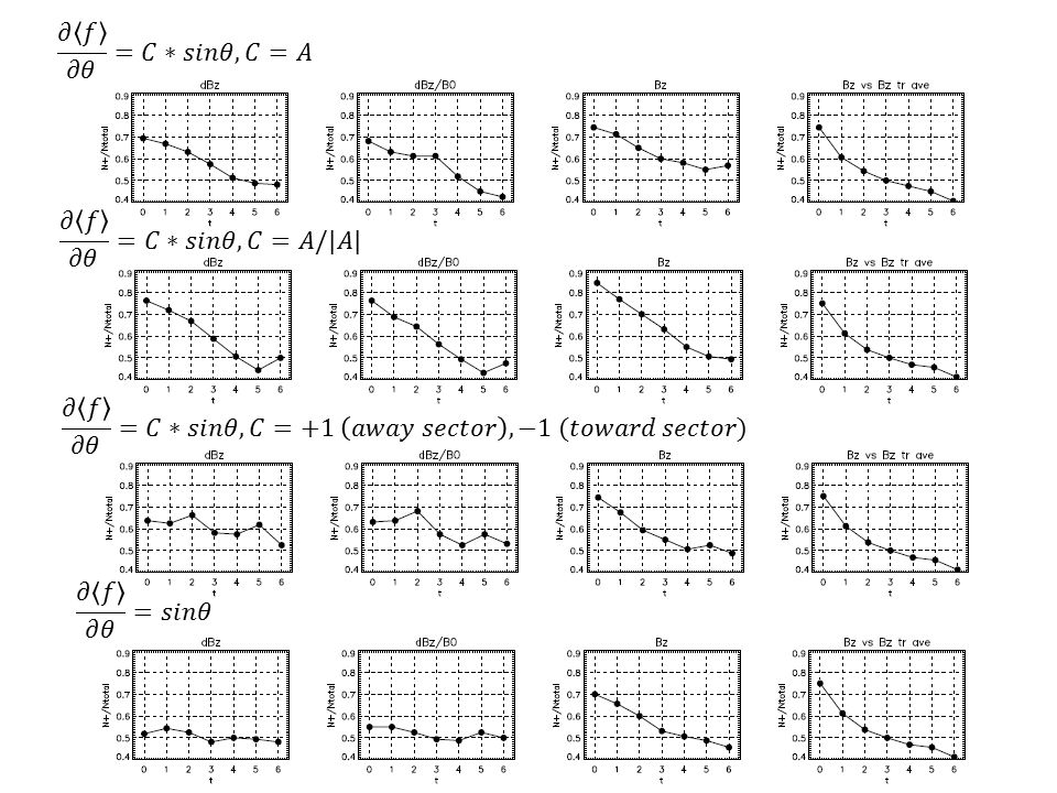
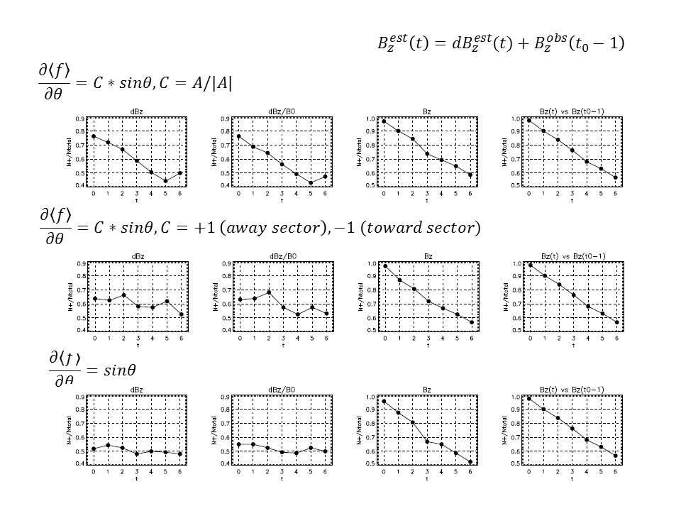
25. Question: why we have good correlation when we use the factor C

26. 0h prediction

31. Update Feb 18 Don’t use the future IMF data for the estimation of future IMF

32. estimation of dB * dB obs is calculated as the deviation from 12-hour tr-moving average of observed IMF in GSE coordinate. * dB exp is calculated from the model in IMF coordinate as Background IMF V sw ·Δt IMF x gse

33. ICME Shock dBz0.3896 dBz/Bt0.3678 Bz0.4533 Bz vs tave of Bz0.1224

36. B0=5nT

37. Update Mar 11

39. 0 hour predict 3 hour predict

41. 0 hour predict 3 hour predict

42. N+/Nall Mean of corr. coeff Median of corr. coeff

43. 6 years of data 0 hour prediction 5 hour prediction

44. 6 years of data (event period only) 0 hour prediction 5 hour prediction

45. 6 years of data (without event period) 0 hour prediction 5 hour prediction