Download presentation
Presentation is loading. Please wait.

1
Automatic selection of reference velocities for recursive depth migration Hugh Geiger and Gary Margrave CREWES Nov 2004

2
POTSI* Sponsors: *Pseudo-differential Operator Theory in Seismic Imaging

3
The problem: Many recursive wavefield extrapolators require a limited set of reference velocities for efficient implementation How should these reference velocities be chosen? example velocity profiles

4
Objectives: Efficient computation - a minimum number of reference velocities Accurate wavefield extrapolation - reference velocities ‘close’ to model velocities too few reference velocities? ~3000 ms -1 (~230%)
.")
5
Some specific requirements PSPI – lower and upper bounding velocities (v min,v max ) - ideally minimize large interpolations (wavefield is a weighted summation) Split-step – more accurate focusing with a slower velocity too many reference velocities? ~80 ms -1 (~ 5%) ~70 ms -1 (~ 4%) ~320 ms -1 (~ 17%) ~40 ms -1 (~ 2%)
 ~70 ms -1 (~ 4%) ~320 ms -1 (~ 17%) ~40 ms -1 (~ 2%).")
6
Basic approach 1: Linear progression choose an approximate velocity spacing dV nV=round((v max -v min )/dV) v step =(v max -v min )/nV what is a good choice for dV? - empirical testing required - reasonable for both low and high velocities? ~500 ms -1 (~20%) ~500 ms -1 (~10%)
 ~500 ms -1 (~10%).")
7
(detail for subsequent figures) Basic approach 2a: Geometric progression choose an appropriate percentage step v prcnt v(i) = (1+v prcnt )*v(i-1) - Kessigner (1992) recommends v prcnt =0.15 - start at v min for profile? - start at v min for complete velocity model? (perhaps if using lookup tables) ~370 ms -1 (~15%) ~750 ms -1 (~15%)
 ~370 ms -1 (~15%) ~750 ms -1 (~15%).")
8
Statistical method of Bagaini et al (1995) choose a preliminary dv (geometric?) equally spaced bins over v min :v max (e.g. nB temp = 6) bin the velocities to give probability density P i, P i = 1 optimal number of bins by statistical entropy S= P i logP i nB opt = round(exp(S)+0.5) (e.g. nB opt = 5)
 bin the velocities to give probability density P i, P i = 1 optimal number of bins by statistical entropy S= P i logP i nB opt = round(exp(S)+0.5) (e.g. nB opt = 5).")
9
calculate cumulative probability distribution Y i, Y i = P i each optimal bin to hold 1/nB opt (e.g. 0.2) - start at v min -linearly interpolate from temporary bin boundaries (e.g. at 0.2, 0.4, 0.6, 0.8) Is this optimal? - bins not necessarily close to peaks
 - start at v min -linearly interpolate from temporary bin boundaries (e.g. at 0.2, 0.4, 0.6, 0.8) Is this optimal. - bins not necessarily close to peaks.")
10
New peak search method cluster velocities - new cluster where jump exceeds v prcntmax Now, within each cluster: use Bagaini method for optimal number of bins nB opt create a new probability distribution with finer bins descending sort of P i ’s, choose all P i ’s where P i < 0.9 place v temp at all P i ’s, include v min,v max use ‘greedy search’ to combine closely spaced P i ’s - start search at bin spacing of 1, then 2, etc. - weighted linear average to move v temp stop when at v temp = nB opt

13
Marmousi bandlimited reflectivity

14
PSPI with velocity clustering algorithm data: deconpr 50 13.0002 whiten [4 16 35 60] static –60ms shot: ricker fdom 24 ghost array phsrot –68 (to zp) whiten [4 16 35 60]
![PSPI with velocity clustering algorithm data: deconpr whiten [ ] static –60ms shot: ricker fdom 24 ghost array phsrot –68 (to zp) whiten [ ]](http://images.slideplayer.com/25/8195324/slides/slide_14.jpg "PSPI with velocity clustering algorithm data: deconpr whiten [ ] static –60ms shot: ricker fdom 24 ghost array phsrot –68 (to zp) whiten [ ]")
15
Marmousi bandlimited reflectivity

16
Marmousi shallow reflectivity

17
Linear

18
Geometric

19
Bagaini

20
Peak Search

21
Modified Bagaini: clusters

22
Marmousi shallow reflectivity

23
Linear

24
Geometric

25
Bagaini

26
Peak Search

27
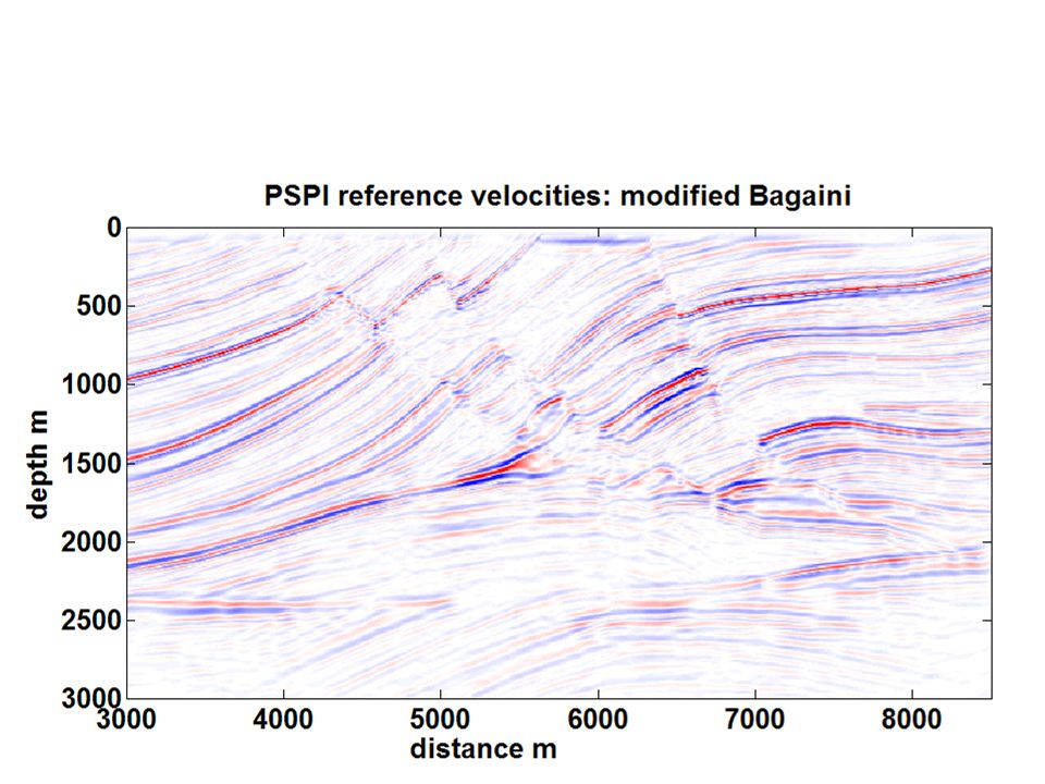
Modified Bagaini: clusters

28
Static shifts – affect focusing

29
a) source wavefield in (x,z,t)b) reflected wavefield in (x,z,t) x z t z x z t c) direct + reflected arrival at z=0d) another perspective of (c) x z t x t (figures courtesy J. Bancroft) horizontal reflector (blue)
 horizontal reflector (blue).")
30
z=0 z=2 z=3 z=4 z=1 x t reflector With a static shift of the source and/or receiver wavefield, the extrpolated wavefields will not be time coincident at the reflector, causing Focusing and positioning errors.

31
rec array source array hard water bottom free surface Complications for Marmousi imaging: free-surface and water bottom ghosting and multiples modify wavelet source and receiver array directivity two-way wavefield, one-way extrapolators heterogeneous velocity

32
220m 32m 28m 0m x=400m v=1500m/s ρ=1000kg/m 3 v=1549m/s ρ=1478kg/m 3 v=1598m/s ρ=1955kg/m 3 v=1598m/s ρ=4000kg/m 3 x=0m Marmousi source array: 6 airguns at 8m spacing, depth 8m receiver array: 5 hydrophones at 4m spacing, depth 12m

33
reflector downgoing transmitted wave upgoing reflected wave receiver array @ 45º receiver array @ 0º Modeled with finite difference code (courtesy Peter Manning) to examine response of isolated reflector at 0 º and ~45 º degree incidence
 to examine response of isolated reflector at 0 º and ~45 º degree incidence")
34
normal incidence reflection ~45 degree incidence reflection ~60ms desired 24 Hz zero-phase Ricker wavelet Marmousi airgun wavelet After free-surface ghosting and water-bottom multiples, the Marmousi airgun wavelet propagates as ~24 Hz zero-phase Ricker with 60 ms delay.

35
The deconvolution chosen for the Marmousi data set is a simple spectral whitening followed by a gap deconvolution (40ms gap, 200ms operator) this yields a reasonable zero phase wavelet in preparation for depth imaging Deconvolution
 this yields a reasonable zero phase wavelet in preparation for depth imaging Deconvolution")
36
the receiver wavefield is then static shifted by -60ms to create an approximate zero phase wavelet if the receiver wavefield is extrapolated and imaged without compensating for the 60ms delay, focusing and positioning are compromised, as illustrated using a simple synthetic for a diffractor diffractor imaging with no delay diffractor imaging with 60ms delay

37
reflectivity x: 4000-6000 z: 0-1000

38
PSPI whiten [4 16 35 60] cvel.2% clip 6 data: deconpr 50 13.0002 whiten [4 16 35 60] static 0ms shot: ricker fdom 24 ghost array phsrot –68 (to zp) unwhiten
![PSPI whiten [ ] cvel.2% clip 6 data: deconpr whiten [ ] static 0ms shot: ricker fdom 24 ghost array phsrot –68 (to zp) unwhiten](http://images.slideplayer.com/25/8195324/slides/slide_38.jpg "PSPI whiten [ ] cvel.2% clip 6 data: deconpr whiten [ ] static 0ms shot: ricker fdom 24 ghost array phsrot –68 (to zp) unwhiten")
39
PSPI whiten [4 16 35 60] cvel.2% clip 6 data: deconpr 50 13.0002 whiten [4 16 35 60] static –16ms shot: ricker fdom 24 ghost array phsrot –68 (to zp) unwhiten
![PSPI whiten [ ] cvel.2% clip 6 data: deconpr whiten [ ] static –16ms shot: ricker fdom 24 ghost array phsrot –68 (to zp) unwhiten](http://images.slideplayer.com/25/8195324/slides/slide_39.jpg "PSPI whiten [ ] cvel.2% clip 6 data: deconpr whiten [ ] static –16ms shot: ricker fdom 24 ghost array phsrot –68 (to zp) unwhiten")
40
PSPI whiten [4 16 35 60] cvel.2% clip 6 data: deconpr 50 13.0002 whiten [4 16 35 60] static –32ms shot: ricker fdom 24 ghost array phsrot –68 (to zp) unwhiten
![PSPI whiten [ ] cvel.2% clip 6 data: deconpr whiten [ ] static –32ms shot: ricker fdom 24 ghost array phsrot –68 (to zp) unwhiten](http://images.slideplayer.com/25/8195324/slides/slide_40.jpg "PSPI whiten [ ] cvel.2% clip 6 data: deconpr whiten [ ] static –32ms shot: ricker fdom 24 ghost array phsrot –68 (to zp) unwhiten")
41
PSPI whiten [4 16 35 60] cvel.02% clip 6 data: deconpr 50 13.0002 whiten [4 16 35 60] static –56ms shot: ricker fdom 24 ghost array phsrot –68 (to zp) unwhiten
![PSPI whiten [ ] cvel.02% clip 6 data: deconpr whiten [ ] static –56ms shot: ricker fdom 24 ghost array phsrot –68 (to zp) unwhiten](http://images.slideplayer.com/25/8195324/slides/slide_41.jpg "PSPI whiten [ ] cvel.02% clip 6 data: deconpr whiten [ ] static –56ms shot: ricker fdom 24 ghost array phsrot –68 (to zp) unwhiten")
42
PSPI whiten [4 16 35 60] cvel.02% clip 6 data: deconpr 50 13.0002 whiten [4 16 35 60] static –56ms shot: ricker fdom 24 ghost array phsrot –45 (to zp) whiten [4 16 35 60]
![PSPI whiten [ ] cvel.02% clip 6 data: deconpr whiten [ ] static –56ms shot: ricker fdom 24 ghost array phsrot –45 (to zp) whiten [ ]](http://images.slideplayer.com/25/8195324/slides/slide_42.jpg "PSPI whiten [ ] cvel.02% clip 6 data: deconpr whiten [ ] static –56ms shot: ricker fdom 24 ghost array phsrot –45 (to zp) whiten [ ]")
43
Marmousi bandlimited reflectivity - shifted to match Zhang et al. (2003)
")
44
Zhang et al. (2003) – positioning not accurate
 – positioning not accurate")
45
PSPI reference velocities: peak search - shifted to match Zhang et al. (2003)
")
46
Marmousi bandlimited reflectivity (as before)
")
47
Marmousi shallow reflectivity

48
Marmousi target reservoir

57
V=3000m/s V=2000m/s cos taper 70°-87.5° PSPI creates discontinuities at boundaries – smoothing may be good!

58
Conclusions Preprocessing to zero phase, shot modeling, and correction of static shifts important for imaging Optimal selection of reference velocities desired to maximize accuracy and efficiency of wavefield extrapolation Linear or geometric progression does not take into account distribution of velocities Bagaini et al. method does not necessarily pick reference velocities close to model velocities New peak search method selects reference velocites close to model velocities

59
Conclusions (cont) However, Bagaini method performs well on Marmousi! Our PSPI implementation provides a good standard for judging our other algorithms

62
(-60ms static + 16.67m down)
")
63
-56ms static + 8.33m down

64
(-56ms static + 8.33m down)
")
65
reflectivity x: 3000-8500 z: 0-3000

67
Shift down 8.33m

68
PSPI whiten [4 16 30 55] cvel.2% clip 4 data: deconpr 50 13.0002 whiten [4 16 35 60] static –60ms shot: ricker fdom 24 ghost array phsrot –68 (to zp) whiten [4 16 35 60]
![PSPI whiten [ ] cvel.2% clip 4 data: deconpr whiten [ ] static –60ms shot: ricker fdom 24 ghost array phsrot –68 (to zp) whiten [ ]](http://images.slideplayer.com/25/8195324/slides/slide_68.jpg "PSPI whiten [ ] cvel.2% clip 4 data: deconpr whiten [ ] static –60ms shot: ricker fdom 24 ghost array phsrot –68 (to zp) whiten [ ]")
Similar presentations


 at the Frio Project T.M. Daley, L.R. Myer*, G.M. Hoversten and E.L. Majer.>")


