Download presentation
Presentation is loading. Please wait.

1
ECE & TCOM 590 Microwave Transmission for Telecommunications Introduction to Microwaves January 29, 2004

2
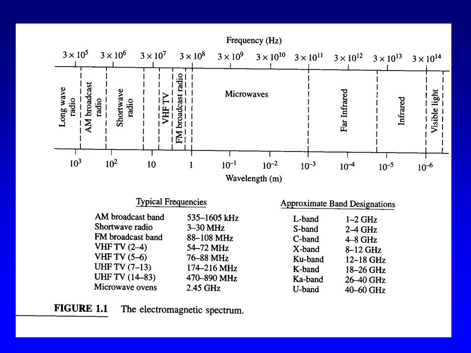
Microwave Applications –Wireless Applications –TV and Radio broadcast –Optical Communications –Radar –Navigation –Remote Sensing –Domestic and Industrial Applications –Medical Applications –Surveillance –Astronomy and Space Exploration

3
Brief Microwave History Maxwell (1864-73) –integrated electricity and magnetism –set of 4 coherent and self-consistent equations –predicted electromagnetic wave propagation Hertz (1873-91) –experimentally confirmed Maxwell’s equations –oscillating electric spark to induce similar oscillations in a distant wire loop ( =10 cm)
 –integrated electricity and magnetism –set of 4 coherent and self-consistent equations –predicted electromagnetic wave propagation Hertz ( ) –experimentally confirmed Maxwell’s equations –oscillating electric spark to induce similar oscillations in a distant wire loop ( =10 cm)")
4
Brief Microwave History Marconi (early 20th century) –parabolic antenna to demonstrate wireless telegraphic communications –tried to commercialize radio at low frequency Lord Rayleigh (1897) –showed mathematically that EM wave propagation possible in waveguides George Southworth (1930) –showed waveguides capable of small bandwidth transmission for high powers
 –parabolic antenna to demonstrate wireless telegraphic communications –tried to commercialize radio at low frequency Lord Rayleigh (1897) –showed mathematically that EM wave propagation possible in waveguides George Southworth (1930) –showed waveguides capable of small bandwidth transmission for high powers")
5
Brief Microwave History R.H. and S.F. Varian (1937) –development of the klystron MIT Radiation Laboratory (WWII) –radiation lab series - classic writings Development of transistor (1950’s) Development of Microwave Integrated Circuits –microwave circuit on a chip –microstrip lines Satellites, wireless communications,...
 –development of the klystron MIT Radiation Laboratory (WWII) –radiation lab series - classic writings Development of transistor (1950’s) Development of Microwave Integrated Circuits –microwave circuit on a chip –microstrip lines Satellites, wireless communications,....")
7
Ref: text by Pozar

8
Microwave Engr. Distinctions ·1 - Circuit Lengths: ·Low frequency ac or rf circuits ·time delay, t, of a signal through a device ·t = L/v « T = 1/f where T=period of ac signal ·but f =v so 1/f= /v ·so L «, I.e. size of circuit is generally much smaller than the wavelength (or propagation times 0) ·Microwaves: L ·propagation times not negligible ·Optics: L»
 ·Microwaves: L ·propagation times not negligible ·Optics: L».")
9
Transit Limitations Consider an FET Source to drain spacing roughly 2.5 microns Apply a 10 GHz signal: –T = 1/f = 10 -10 = 0.10 nsec –transit time across S to D is roughly 0.025 nsec or 1/4 of a period so the gate voltage is low and may not permit the S to D current to flow

10
Microwave Distinctions ·2 - Skin Depth: ·degree to which electromagnetic field penetrates a conducting material ·microwave currents tend to flow along the surface of conductors ·so resistive effect is increased, i.e. ·R R DC a / 2 , where – = skin depth = 1/ ( f o cond ) 1/2 –where, R DC = 1 / ( a 2 cond ) –a = radius of the wire R waves in Cu >R low freq. in Cu
 1/2 –where, R DC = 1 / ( a 2 cond ) –a = radius of the wire R waves in Cu >R low freq. in Cu.")
11
Microwave Engr. Distinctions ·3 - Measurement Technique ·At low frequencies circuit properties measured by voltage and current ·But at microwaves frequencies, voltages and currents are not uniquely defined; so impedance and power are measured rather than voltage and current

12
Circuit Limitations Simple circuit: 10V, ac driven, copper wire, #18 guage, 1 inch long and 1 mm in diameter: dc resistance is 0.4 m and inductance is 0.027 H –f = 0; X L = 2 f L 0.18 f 10 -6 =0 –f = 60 Hz; X L 10 -5 = 0.01 m –f = 6 MHz; X L 1 –f = 6 GHz; X L 10 3 = 1 k –So, wires and printed circuit boards cannot be used to connect microwave devices; we need transmission lines

13
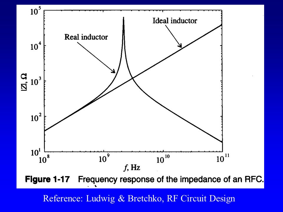
High-Frequency Resistors Inductance and resistance of wire resistors under high-frequency conditions (f 500 MHz): – L/R DC a / (2 ) –R /R DC a / (2 ) –where, R DC = /( a 2 cond ) {the 2 here accounts for 2 leads} –a = radius of the wire – = length of the leads – = skin depth = 1/ ( f o cond ) 1/2
: – L/R DC a / (2 ) –R /R DC a / (2 ) –where, R DC = /( a 2 cond ) {the 2 here accounts for 2 leads} –a = radius of the wire – = length of the leads – = skin depth = 1/ ( f o cond ) 1/2")
14
Reference: Ludwig & Bretchko, RF Circuit Design

15
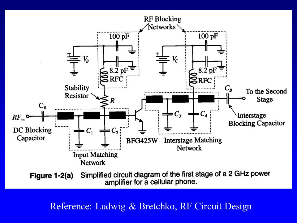
High Frequency Capacitor Equivalent circuit consists of parasitic lead conductance L, series resistance R s describing the losses in the the lead conductors and dielectric loss resistance R e = 1/G e (in parallel) with the Capacitor. G e = C tan s, where –tan s = ( / diel ) -1 = loss tangent
 -1 = loss tangent.")
16
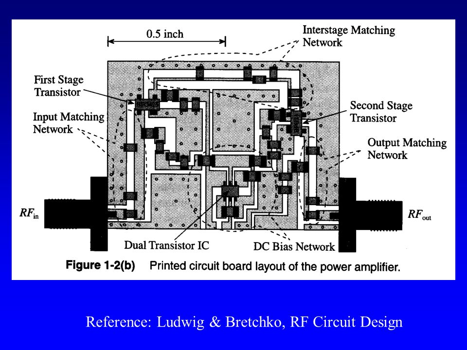
Reference: Ludwig & Bretchko, RF Circuit Design

20
Maxwell’s Equations Gauss No Magnetic Poles Faraday’s Laws Ampere’s Circuit Law

21
Characteristics of Medium Constitutive Relationships

22
Fields in a Dielectric Materials

23
Fields in a Conductive Materials

24
Wave Equation

25
General Procedure to Find Fields in a Guided Structure 1- Use wave equations to find the z component of E z and/or H z –note classifications –TEM: E z = H z = 0 –TE: E z = 0, H z 0 –TM: H z = 0, E z 0 –HE or Hybrid: E z 0, H z 0

26
General Procedure to Find Fields in a Guided Structure 2- Use boundary conditions to solve for any constraints in our general solution for E z and/or H z

27
Plane Waves in Lossless Medium

28
Phase Velocity

29
Wave Impedance

30
Plane Waves in a Lossy Medium

31
Wave Impedance in Lossy Medium

32
Plane Waves in a good Conductor

33
Energy and Power

Similar presentations


>")


![L 28 Electricity and Magnetism [6] magnetism Faraday’s Law of Electromagnetic Induction –induced currents –electric generator –eddy currents Electromagnetic.](/15/4611258/big_thumb.jpg "L 28 Electricity and Magnetism [6] magnetism Faraday’s Law of Electromagnetic Induction –induced currents –electric generator –eddy currents Electromagnetic.>")


>")