Download presentation
Presentation is loading. Please wait.

1
Graphical models, belief propagation, and Markov random fields Bill Freeman, MIT Fredo Durand, MIT 6.882 March 21, 2005

2
Color selection problem (see Photoshop demonstration)
")
3
Stereo problem L R d Squared difference, (L[x] – R[x-d])^2, for some x. Showing local disparity evidence vectors for a set of neighboring positions, x. x d
![Stereo problem L R d Squared difference, (L[x] – R[x-d])^2, for some x.](http://images.slideplayer.com/25/7647497/slides/slide_3.jpg "Showing local disparity evidence vectors for a set of neighboring positions, x. x d.")
4
Super-resolution image synthesis How select which selection of high resolution patches best fits together? Ignoring which patch fits well with which gives this result for the high frequency components of an image:

5
Things we want to be able to articulate in a spatial prior Favor neighboring pixels having the same state (state, meaning: estimated depth, or group segment membership) Favor neighboring nodes have compatible states (a patch at node i should fit well with selected patch at node j). But encourage state changes to occur at certain places (like regions of high image gradient).
..")
6
Graphical models: tinker toys to build complex probability distributions http://mark.michaelis.net/weblog/2002/12/29/Tinker%20Toys%20Car.jpg Circles represent random variables. Lines represent statistical dependencies. There is a corresponding equation that gives P(x1, x2, x3, y, z), but often it’s easier to understand things from the picture. These tinker toys for probabilities let you build up, from simple, easy-to-understand pieces, complicated probability distributions involving many variables. x1x2x3 yz
, but often it’s easier to understand things from the picture. These tinker toys for probabilities let you build up, from simple, easy-to-understand pieces, complicated probability distributions involving many variables. x1x2x3 yz.")
7
Steps in building and using graphical models First, define the function you want to optimize. Note the two common ways of framing the problem –In terms of probabilities. Multiply together component terms, which typically involve exponentials. –In terms of energies. The log of the probabilities. Typically add together the exponentiated terms from above. The second step: optimize that function. For probabilities, take the mean or the max (or use some other “loss function”). For energies, take the min. 3rd step: in many cases, you want to learn the function from the 1 st step.
. For energies, take the min. 3rd step: in many cases, you want to learn the function from the 1 st step..")
8
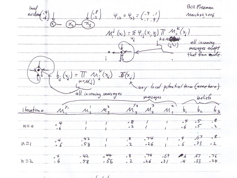
Define model parameters

9
A more general compatibility matrix (values shown as grey scale)
")
10
y1y1 Derivation of belief propagation x1x1 y2y2 x2x2 y3y3 x3x3

11
The posterior factorizes y1y1 x1x1 y2y2 x2x2 y3y3 x3x3

12
Propagation rules y1y1 x1x1 y2y2 x2x2 y3y3 x3x3

13
y1y1 x1x1 y2y2 x2x2 y3y3 x3x3

14
y1y1 x1x1 y2y2 x2x2 y3y3 x3x3

15
Belief propagation: the nosey neighbor rule “Given everything that I know, here’s what I think you should think” (Given the probabilities of my being in different states, and how my states relate to your states, here’s what I think the probabilities of your states should be)
")
16
Belief propagation messages ji i = j To send a message: Multiply together all the incoming messages, except from the node you’re sending to, then multiply by the compatibility matrix and marginalize over the sender’s states. A message: can be thought of as a set of weights on each of your possible states

17
Beliefs j To find a node’s beliefs: Multiply together all the messages coming in to that node.

18
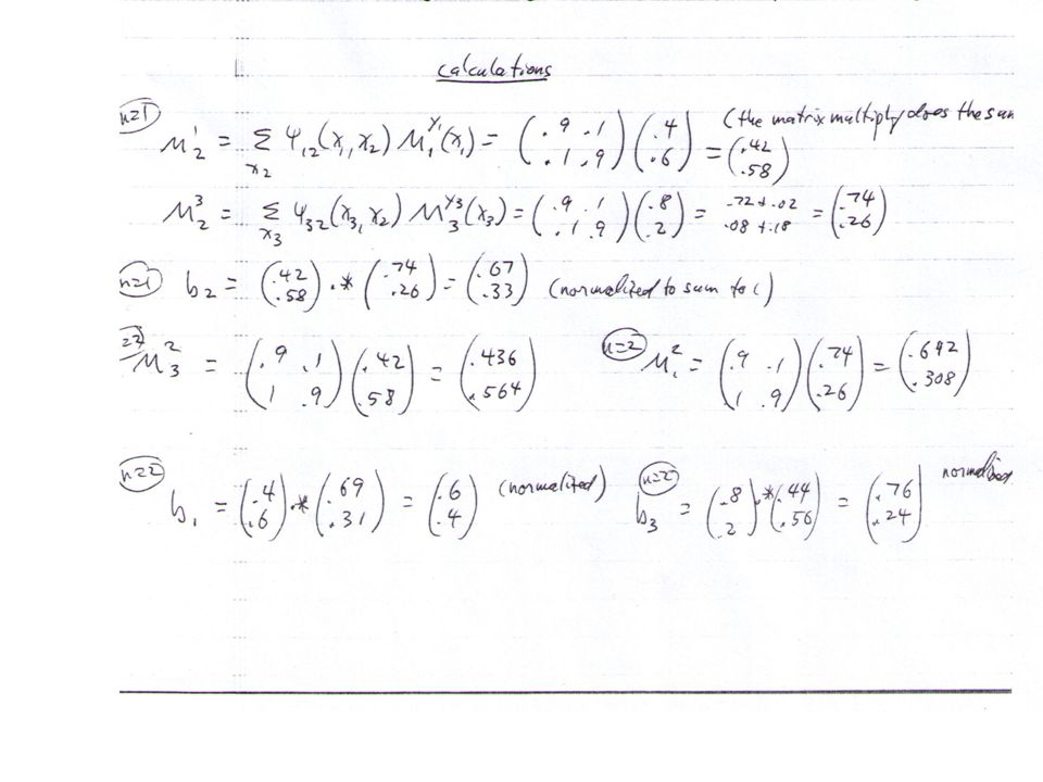
Simple BP example y1y1 x1x1 x2x2 y3y3 x3x3 x1x1 x2x2 x3x3

19
x1x1 x2x2 x3x3 To find the marginal probability for each variable, you can (a)Marginalize out the other variables of: (b)Or you can run belief propagation, (BP). BP redistributes the various partial sums, leading to a very efficient calculation.

22
Belief, and message updates ji i = j

23
Optimal solution in a chain or tree: Belief Propagation “Do the right thing” Bayesian algorithm. For Gaussian random variables over time: Kalman filter. For hidden Markov models: forward/backward algorithm (and MAP variant is Viterbi).
..")
24
Making probability distributions modular, and therefore tractable: Probabilistic graphical models Vision is a problem involving the interactions of many variables: things can seem hopelessly complex. Everything is made tractable, or at least, simpler, if we modularize the problem. That’s what probabilistic graphical models do, and let’s examine that. Readings: Jordan and Weiss intro article—fantastic! Kevin Murphy web page—comprehensive and with pointers to many advanced topics

25
A toy example Suppose we have a system of 5 interacting variables, perhaps some are observed and some are not. There’s some probabilistic relationship between the 5 variables, described by their joint probability, P(x1, x2, x3, x4, x5). If we want to find out what the likely state of variable x1 is (say, the position of the hand of some person we are observing), what can we do? Two reasonable choices are: (a) find the value of x1 (and of all the other variables) that gives the maximum of P(x1, x2, x3, x4, x5); that’s the MAP solution. Or (b) marginalize over all the other variables and then take the mean or the maximum of the other variables. Marginalizing, then taking the mean, is equivalent to finding the MMSE solution. Marginalizing, then taking the max, is called the max marginal solution and sometimes a useful thing to do.
. If we want to find out what the likely state of variable x1 is (say, the position of the hand of some person we are observing), what can we do. Two reasonable choices are: (a) find the value of x1 (and of all the other variables) that gives the maximum of P(x1, x2, x3, x4, x5); that’s the MAP solution. Or (b) marginalize over all the other variables and then take the mean or the maximum of the other variables. Marginalizing, then taking the mean, is equivalent to finding the MMSE solution. Marginalizing, then taking the max, is called the max marginal solution and sometimes a useful thing to do..")
26
To find the marginal probability at x1, we have to take this sum: If the system really is high dimensional, that will quickly become intractable. But if there is some modularity in then things become tractable again. Suppose the variables form a Markov chain: x1 causes x2 which causes x3, etc. We might draw out this relationship as follows:

27
By the chain rule, for any probability distribution, we have: Now our marginalization summations distribute through those terms: P(a,b) = P(b|a) P(a) But if we exploit the assumed modularity of the probability distribution over the 5 variables (in this case, the assumed Markov chain structure), then that expression simplifies:
 = P(b|a) P(a) But if we exploit the assumed modularity of the probability distribution over the 5 variables (in this case, the assumed Markov chain structure), then that expression simplifies:")
28
Belief propagation Performing the marginalization by doing the partial sums is called “belief propagation”. In this example, it has saved us a lot of computation. Suppose each variable has 10 discrete states. Then, not knowing the special structure of P, we would have to perform 10000 additions (10^4) to marginalize over the four variables. But doing the partial sums on the right hand side, we only need 40 additions (10*4) to perform the same marginalization!
 to marginalize over the four variables. But doing the partial sums on the right hand side, we only need 40 additions (10*4) to perform the same marginalization!.")
29
Another modular probabilistic structure, more common in vision problems, is an undirected graph: The joint probability for this graph is given by: Where is called a “compatibility function”. We can define compatibility functions we result in the same joint probability as for the directed graph described in the previous slides; for that example, we could use either form.

30
No factorization with loops! y1y1 x1x1 y2y2 x2x2 y3y3 x3x3 31 ),(xx
,(xx ")
31
Justification for running belief propagation in networks with loops Experimental results: –Error-correcting codes –Vision applications Theoretical results: –For Gaussian processes, means are correct. –Large neighborhood local maximum for MAP. –Equivalent to Bethe approx. in statistical physics. –Tree-weighted reparameterization Weiss and Freeman, 2000 Yedidia, Freeman, and Weiss, 2000 Freeman and Pasztor, 1999; Frey, 2000 Kschischang and Frey, 1998; McEliece et al., 1998 Weiss and Freeman, 1999 Wainwright, Willsky, Jaakkola, 2001

32
Region marginal probabilities i ji

33
Belief propagation equations Belief propagation equations come from the marginalization constraints. jii ji i =

34
Results from Bethe free energy analysis Fixed point of belief propagation equations iff. Bethe approximation stationary point. Belief propagation always has a fixed point. Connection with variational methods for inference: both minimize approximations to Free Energy, –variational: usually use primal variables. –belief propagation: fixed pt. equs. for dual variables. Kikuchi approximations lead to more accurate belief propagation algorithms. Other Bethe free energy minimization algorithms— Yuille, Welling, etc.

35
Kikuchi message-update rules i ji = ji ji lk = Groups of nodes send messages to other groups of nodes. Update for messages Update for messages Typical choice for Kikuchi cluster.

36
Generalized belief propagation Marginal probabilities for nodes in one row of a 10x10 spin glass BP: belief propagation GBP: generalized belief propagation ML: maximum likelihood

37
References on BP and GBP J. Pearl, 1985 –classic Y. Weiss, NIPS 1998 –Inspires application of BP to vision W. Freeman et al learning low-level vision, IJCV 1999 –Applications in super-resolution, motion, shading/paint discrimination H. Shum et al, ECCV 2002 –Application to stereo M. Wainwright, T. Jaakkola, A. Willsky –Reparameterization version J. Yedidia, AAAI 2000 –The clearest place to read about BP and GBP.

38
Probability models for entire images: Markov Random Fields Allows rich probabilistic models for images. But built in a local, modular way. Learn local relationships, get global effects out.

39
MRF nodes as pixels Winkler, 1995, p. 32

40
MRF nodes as patches image patches (x i, y i ) (x i, x j ) image scene scene patches
 (x i, x j ) image scene scene patches")
41
Network joint probability scene image Scene-scene compatibility function neighboring scene nodes local observations Image-scene compatibility function i ii ji ji yxxx Z yxP),(),( 1 ),(,
,(),( 1 ),(,")
42
In order to use MRFs: Given observations y, and the parameters of the MRF, how infer the hidden variables, x? How learn the parameters of the MRF?

43
Outline of MRF section Inference in MRF’s. –Iterated conditional modes (ICM) –Gibbs sampling, simulated annealing –Variational methods –Belief propagation –Graph cuts Vision applications of inference in MRF’s. Learning MRF parameters. –Iterative proportional fitting (IPF)
 –Gibbs sampling, simulated annealing –Variational methods –Belief propagation –Graph cuts Vision applications of inference in MRF’s. Learning MRF parameters. –Iterative proportional fitting (IPF).")
44
Iterated conditional modes For each node: –Condition on all the neighbors –Find the mode –Repeat. Described in: Winkler, 1995. Introduced by Besag in 1986.

45
Winkler, 1995

46
Outline of MRF section Inference in MRF’s. –Iterated conditional modes (ICM) –Gibbs sampling, simulated annealing –Variational methods –Belief propagation –Graph cuts Vision applications of inference in MRF’s. Learning MRF parameters. –Iterative proportional fitting (IPF)
 –Gibbs sampling, simulated annealing –Variational methods –Belief propagation –Graph cuts Vision applications of inference in MRF’s. Learning MRF parameters. –Iterative proportional fitting (IPF).")
47
Gibbs Sampling and Simulated Annealing Gibbs sampling: –A way to generate random samples from a (potentially very complicated) probability distribution. Simulated annealing: –A schedule for modifying the probability distribution so that, at “zero temperature”, you draw samples only from the MAP solution. Reference: Geman and Geman, IEEE PAMI 1984.

48
Sampling from a 1-d function 1.Discretize the density function 2. Compute distribution function from density function 3. Sampling draw ~ U(0,1); for k = 1 to n if break; ;
; for k = 1 to n if break; ;.")
49
Gibbs Sampling x1x1 x2x2 Slide by Ce Liu

50
Gibbs sampling and simulated annealing Simulated annealing as you gradually lower the “temperature” of the probability distribution ultimately giving zero probability to all but the MAP estimate. What’s good about it: finds global MAP solution. What’s bad about it: takes forever. Gibbs sampling is in the inner loop…

51
Gibbs sampling and simulated annealing So you can find the mean value (MMSE estimate) of a variable by doing Gibbs sampling and averaging over the values that come out of your sampler. You can find the MAP value of a variable by doing Gibbs sampling and gradually lowering the temperature parameter to zero.

52
Outline of MRF section Inference in MRF’s. –Iterated conditional modes (ICM) –Gibbs sampling, simulated annealing –Variational methods –Belief propagation –Graph cuts Vision applications of inference in MRF’s. Learning MRF parameters. –Iterative proportional fitting (IPF)
 –Gibbs sampling, simulated annealing –Variational methods –Belief propagation –Graph cuts Vision applications of inference in MRF’s. Learning MRF parameters. –Iterative proportional fitting (IPF).")
53
Variational methods Reference: Tommi Jaakkola’s tutorial on variational methods, http://www.ai.mit.edu/people/tommi/ Example: mean field –For each node Calculate the expected value of the node, conditioned on the mean values of the neighbors.

54
Outline of MRF section Inference in MRF’s. –Iterated conditional modes (ICM) –Gibbs sampling, simulated annealing –Variational methods –Belief propagation –Graph cuts Vision applications of inference in MRF’s. Learning MRF parameters. –Iterative proportional fitting (IPF)
 –Gibbs sampling, simulated annealing –Variational methods –Belief propagation –Graph cuts Vision applications of inference in MRF’s. Learning MRF parameters. –Iterative proportional fitting (IPF).")
55
Outline of MRF section Inference in MRF’s. –Iterated conditional modes (ICM) –Gibbs sampling, simulated annealing –Variational methods –Belief propagation –Graph cuts Vision applications of inference in MRF’s. Learning MRF parameters. –Iterative proportional fitting (IPF)
 –Gibbs sampling, simulated annealing –Variational methods –Belief propagation –Graph cuts Vision applications of inference in MRF’s. Learning MRF parameters. –Iterative proportional fitting (IPF).")
56
Graph cuts Algorithm: uses node label swaps or expansions as moves in the algorithm to reduce the energy. Swaps many labels at once, not just one at a time, as with ICM. Find which pixel labels to swap using min cut/max flow algorithms from network theory. Can offer bounds on optimality. See Boykov, Veksler, Zabih, IEEE PAMI 23 (11) Nov. 2001 (available on web).
 Nov (available on web)..")
57
Comparison of graph cuts and belief propagation Comparison of Graph Cuts with Belief Propagation for Stereo, using Identical MRF Parameters, ICCV 2003. Marshall F. Tappen William T. Freeman

58
Ground truth, graph cuts, and belief propagation disparity solution energies

59
Graph cuts versus belief propagation Graph cuts consistently gave slightly lower energy solutions for that stereo-problem MRF, although BP ran faster, although there is now a faster graph cuts implementation than what we used… However, here’s why I still use Belief Propagation: –Works for any compatibility functions, not a restricted set like graph cuts. –I find it very intuitive. –Extensions: sum-product algorithm computes MMSE, and Generalized Belief Propagation gives you very accurate solutions, at a cost of time.

60
MAP versus MMSE

61
Show program comparing some methods on a simple MRF testMRF.m

62
Outline of MRF section Inference in MRF’s. –Gibbs sampling, simulated annealing –Iterated condtional modes (ICM) –Variational methods –Belief propagation –Graph cuts Applications of inference in MRF’s. Learning MRF parameters. –Iterative proportional fitting (IPF)
 –Variational methods –Belief propagation –Graph cuts Applications of inference in MRF’s. Learning MRF parameters. –Iterative proportional fitting (IPF).")
63
Applications of MRF’s Stereo Motion estimation Labelling shading and reflectance Many others…

64
Applications of MRF’s Stereo Motion estimation Labelling shading and reflectance Many others…

65
Motion application image patches image scene scene patches

66
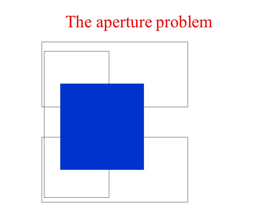
What behavior should we see in a motion algorithm? Aperture problem Resolution through propagation of information Figure/ground discrimination

67
The aperture problem

69
Program demo

70
Motion analysis: related work Markov network –Luettgen, Karl, Willsky and collaborators. Neural network or learning-based –Nowlan & T. J. Senjowski; Sereno. Optical flow analysis –Weiss & Adelson; Darrell & Pentland; Ju, Black & Jepson; Simoncelli; Grzywacz & Yuille; Hildreth; Horn & Schunk; etc.

71
Motion estimation results (maxima of scene probability distributions displayed) Initial guesses only show motion at edges. Iterations 0 and 1 Inference: Image data

72
Motion estimation results Figure/ground still unresolved here. (maxima of scene probability distributions displayed) Iterations 2 and 3
 Iterations 2 and 3.")
73
Motion estimation results Final result compares well with vector quantized true (uniform) velocities. (maxima of scene probability distributions displayed) Iterations 4 and 5
 Iterations 4 and 5.")
74
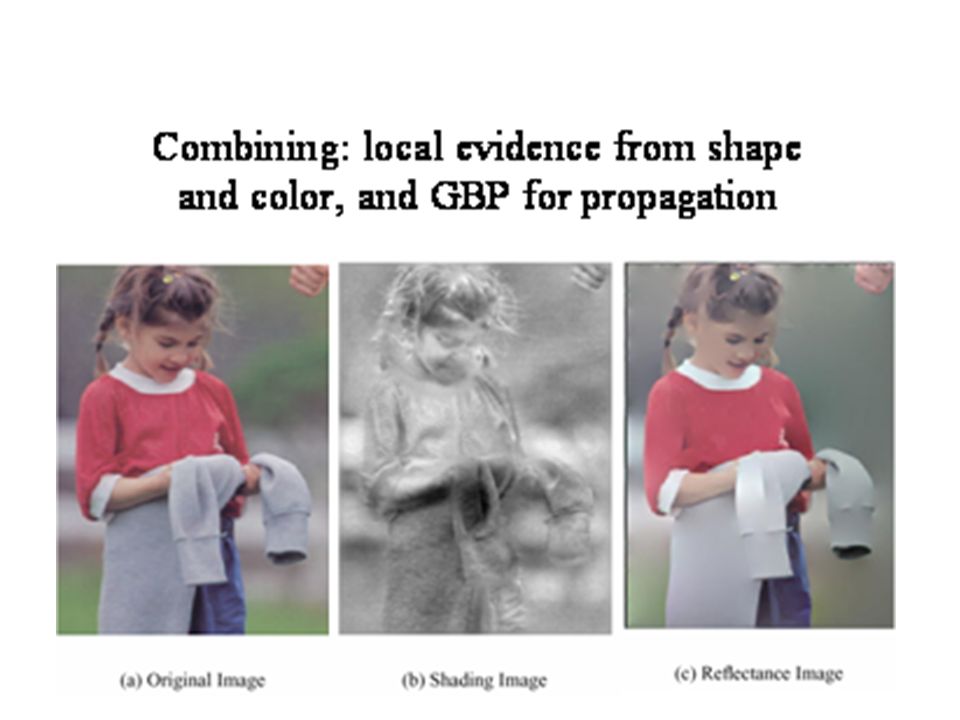
Vision applications of MRF’s Stereo Motion estimation Labelling shading and reflectance Many others…

75
Forming an Image Surface (Height Map) Illuminate the surface to get: The shading image is the interaction of the shape of the surface and the illumination Shading Image
 Illuminate the surface to get: The shading image is the interaction of the shape of the surface and the illumination Shading Image")
76
Painting the Surface Scene Add a reflectance pattern to the surface. Points inside the squares should reflect less light Image

77
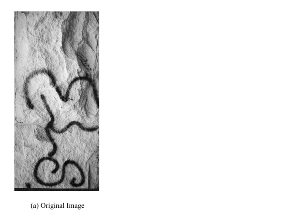
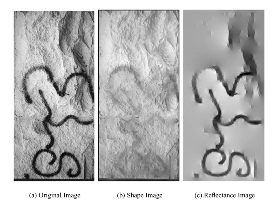
Goal Image Shading Image Reflectance Image

78
Basic Steps 1.Compute the x and y image derivatives 2.Classify each derivative as being caused by either shading or a reflectance change 3.Set derivatives with the wrong label to zero. 4.Recover the intrinsic images by finding the least- squares solution of the derivatives. Original x derivative image Classify each derivative (White is reflectance)
.")
79
Learning the Classifiers Combine multiple classifiers into a strong classifier using AdaBoost (Freund and Schapire) Choose weak classifiers greedily similar to (Tieu and Viola 2000) Train on synthetic images Assume the light direction is from the right Shading Training Set Reflectance Change Training Set
 Choose weak classifiers greedily similar to (Tieu and Viola 2000) Train on synthetic images Assume the light direction is from the right Shading Training Set Reflectance Change Training Set")
80
Using Both Color and Gray-Scale Information Results without considering gray-scale

81
Some Areas of the Image Are Locally Ambiguous Input Shading Reflectance Is the change here better explained as or ?

82
Propagating Information Can disambiguate areas by propagating information from reliable areas of the image into ambiguous areas of the image

83
Consider relationship between neighboring derivatives Use Generalized Belief Propagation to infer labels Propagating Information

84
Setting Compatibilities Set compatibilities according to image contours –All derivatives along a contour should have the same label Derivatives along an image contour strongly influence each other 0.51.0 β=β=

85
Improvements Using Propagation Input Image Reflectance Image With Propagation Reflectance Image Without Propagation

87
(More Results) Input ImageShading Image Reflectance Image
 Input ImageShading Image Reflectance Image")
90
Outline of MRF section Inference in MRF’s. –Gibbs sampling, simulated annealing –Iterated conditional modes (ICM) –Variational methods –Belief propagation –Graph cuts Vision applications of inference in MRF’s. Learning MRF parameters. –Iterative proportional fitting (IPF)
 –Variational methods –Belief propagation –Graph cuts Vision applications of inference in MRF’s. Learning MRF parameters. –Iterative proportional fitting (IPF).")
91
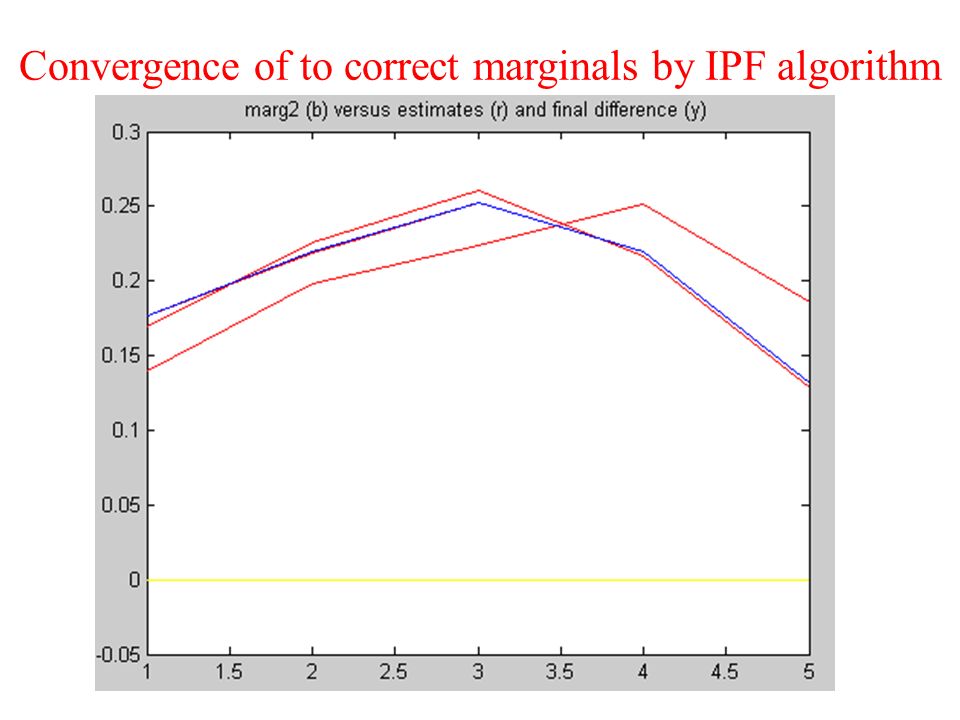
Learning MRF parameters, labeled data Iterative proportional fitting lets you make a maximum likelihood estimate a joint distribution from observations of various marginal distributions.

92
True joint probability Observed marginal distributions

93
Initial guess at joint probability

94
IPF update equation Scale the previous iteration’s estimate for the joint probability by the ratio of the true to the predicted marginals. Gives gradient ascent in the likelihood of the joint probability, given the observations of the marginals. See: Michael Jordan’s book on graphical models

95
Convergence of to correct marginals by IPF algorithm

97
IPF results for this example: comparison of joint probabilities Initial guess Final maximum entropy estimate True joint probability

98
Application to MRF parameter estimation Can show that for the ML estimate of the clique potentials, c (x c ), the empirical marginals equal the model marginals, This leads to the IPF update rule for c (x c ) Performs coordinate ascent in the likelihood of the MRF parameters, given the observed data. Reference: unpublished notes by Michael Jordan

99
More general graphical models than MRF grids In this course, we’ve studied Markov chains, and Markov random fields, but, of course, many other structures of probabilistic models are possible and useful in computer vision. For a nice on-line tutorial about Bayes nets, see Kevin Murphy’s tutorial in his web page.

100
GrabCut http://research.microsoft.com/vision/Cambridge/papers/siggraph04.pdf

101
end

Similar presentations


 Varun Ganapathi, David Vickrey, John Duchi, Daphne Koller Stanford University TexPoint fonts used.>")

 We want to make some.>")
 (Slides from Sam Roweis)>")


