Download presentation
Presentation is loading. Please wait.

1
Spatial Data Analysis Iowa County Land Values (1926)
")
2
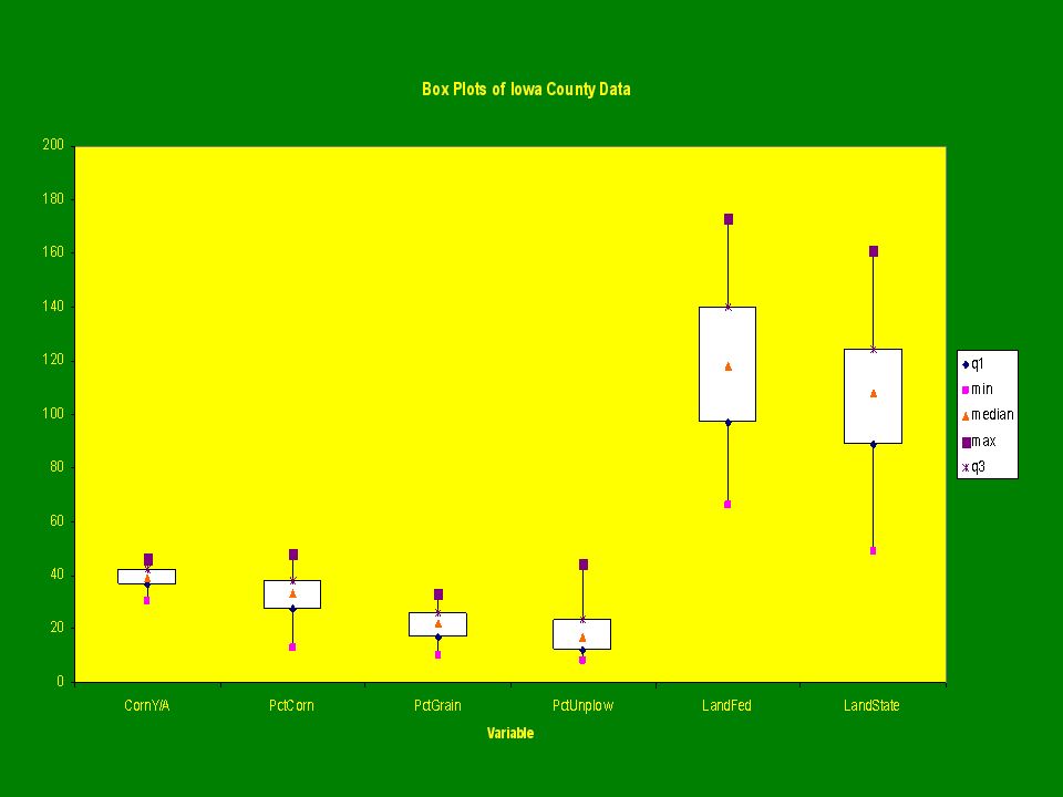
Data Description County Level Data (Circa 1926, n=99) Latitude/Longitude Co-Ordinates of County Seat Land Values per Acre (Federal/State) Corn Yield per Acre Percent Corn Percent Other Grains Percent Un-plowable Land
 Latitude/Longitude Co-Ordinates of County Seat Land Values per Acre (Federal/State) Corn Yield per Acre Percent Corn Percent Other Grains Percent Un-plowable Land")
3
Map of Federal Land Values

4
Summary Statistics StatisticCorn Yield/AcrePercent CornPercent GrainPercent Un-plowFederal ValueState Value q136.527.517129788.5 min30131086649 median39332217118108 max46483344173161 q342382623.5140124 Mean39.1132.4721.5618.85118.68106.25 Std Dev3.407.095.987.8326.7324.38

7
Weight Matrices We consider 2 weight matrices: Inverse distance: Queen’s Case: Each is scaled to have rows sum to 1 with W ii =0

9
Test for Autocorrelation Moran’s I statistic under Randomization:

10
Moran’s I – Federal Land (Queen’s W) N = 99 Counties S 0 = 99 (Rows sum to 1) S 1 = 34.82809 S 2 = 400.6013 k = 2.6268 e’We = 45395.6967 e’e = 70033.6566 I = 0.6482 E(I) = -0.0102 V(I) = 0.003373 Z obs = 11.34
 N = 99 Counties S 0 = 99 (Rows sum to 1) S 1 = S 2 = k = e’We = e’e = I = E(I) = V(I) = Z obs = 11.34")
11
Moran’s I – Federal Land (Inverse Distance) N = 99 Counties S 0 = 99 (Rows sum to 1) S 1 = 3.2919 S 2 = 397.1385 k = 2.0925 e’We = 9772.80233 e’e = 70033.6566 I = 0.1395 E(I) = -0.0102 V(I) = 0.00012972 Z obs = 13.15
 N = 99 Counties S 0 = 99 (Rows sum to 1) S 1 = S 2 = k = e’We = e’e = I = E(I) = V(I) = Z obs = 13.15")
12
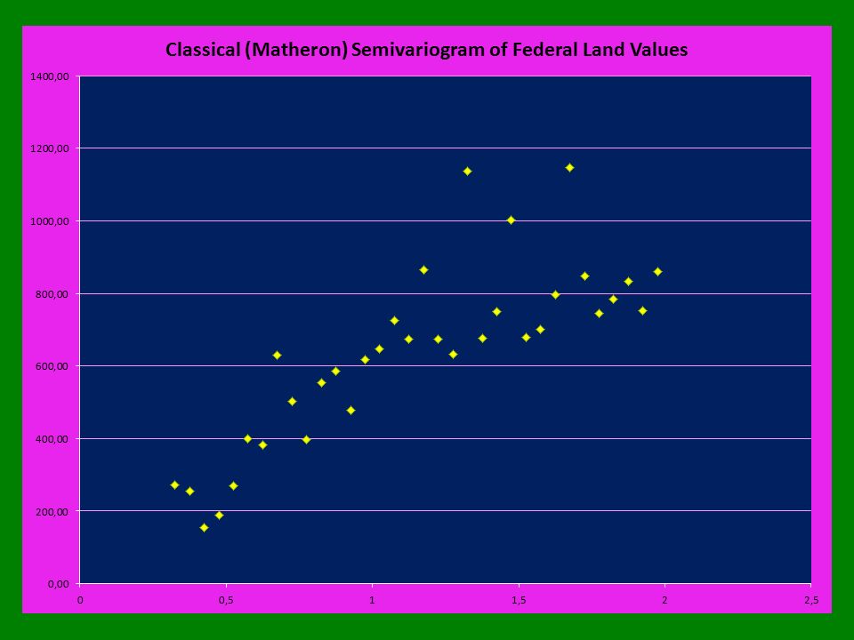
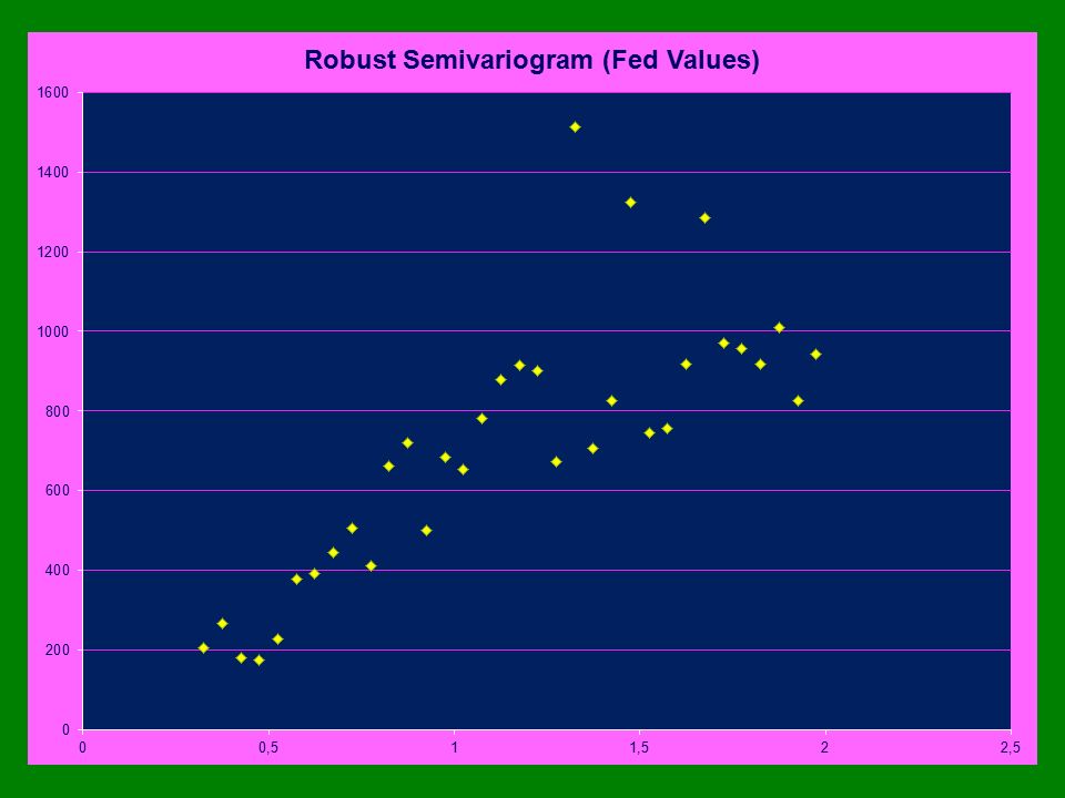
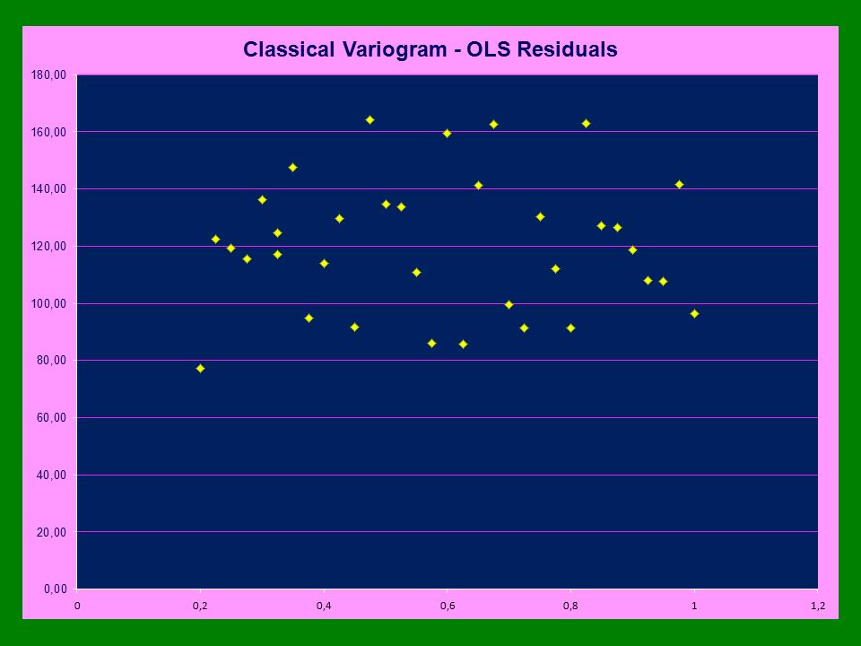
SemiVariogram Estimates Counties assigned to 34 distance classes: <0.35,0.40 to 2.00 by 0.05

15
Several Semivariogram Models

16
Fitted Semivariograms – (R gstat)
")
17
Regression Model Response: FEDVAL = Federal land value Predictors: CORNYLD = Corn yield/acre PCTCORN = Percent of land planted corn PCTGRAIN = Percent of land for other grains PCTUNPLOW = Percent land un-plowable

18
Regression Output Federal land values are: Positively associated with corn yield per acre Positively associated with percent of land planted corn Positively associated with percent of land planted other grains Negatively associated with percent of land un-plowable No evidence of autocorrelated residuals (see following slides)
")
19
Moran’s I – Residuals (Queen’s W) N = 99 Counties S 0 = 99 (Rows sum to 1) S 1 = 34.82809 S 2 = 400.6013 k = 4.1487 e’We = 998.2657 e’e = 12677.997 I = 0.07874 E(I) = -0.0102 V(I) = 0.00330 Z obs = 1.548
 N = 99 Counties S 0 = 99 (Rows sum to 1) S 1 = S 2 = k = e’We = e’e = I = E(I) = V(I) = Z obs = 1.548")
20
Moran’s I – Residuals (Inverse Distance) N = 99 Counties S 0 = 99 (Rows sum to 1) S 1 = 3.2919 S 2 = 397.1385 k = 4.1487 e’We = 91.9083 e’e = 12677.997 I = 0.00725 E(I) = -0.0102 V(I) = 0.00012693 Z obs = 1.549
 N = 99 Counties S 0 = 99 (Rows sum to 1) S 1 = S 2 = k = e’We = e’e = I = E(I) = V(I) = Z obs = 1.549")
22
Map of OLS Residuals

Similar presentations


>")


. Provided by Dr. An Li, San Diego State University.>")