Download presentation
Presentation is loading. Please wait.

1
Spatial Autocorrelation and Spatial Regression
Elisabeth Root Department of Geography

2
A few good books… Bivand, R., E.J. Pebesma and V. Gomez-Rubio. Applied Spatial Data Analysis with R. New York: Springer. Ward, M.D. and K.S. Gleditsch (2008). Spatial Regression Models. Thousand Oaks, CA: Sage.
. Spatial Regression Models. Thousand Oaks, CA: Sage.")
3
First, a note on spatial data
Point data Accuracy of location is very important Area/lattice data Data reported for some regular or irregular areal unit 2 key components of spatial data: Attribute data Spatial data

4
Tobler’s First Law of Geography
“All places are related but nearby places are more related than distant places” Spatial autocorrelation is the formal property that measures the degree to which near and distant things are related Statistical test of match between locational similarity and attribute similarity Positive, negative or zero relationship

5
Spatial regression Steps in determining the extent of spatial autocorrelation in your data and running a spatial regression: Choose a neighborhood criterion Which areas are linked? Assign weights to the areas that are linked Create a spatial weights matrix Run statistical test to examine spatial autocorrelation Run a OLS regression Determine what type of spatial regression to run Run a spatial regression Apply weights matrix

6
Let’s start with spatial autocorrelation

7
Spatial weights matrices
Neighborhoods can be defined in a number of ways Contiguity (common boundary) What is a “shared” boundary? Distance (distance band, K-nearest neighbors) How many “neighbors” to include, what distance do we use? General weights (social distance, distance decay)
 What is a shared boundary Distance (distance band, K-nearest neighbors) How many neighbors to include, what distance do we use General weights (social distance, distance decay)")
8
Step 1: Choose a neighborhood criterion
Importing shapefiles into R and constructing neighborhood sets

9
R libraries we’ll use SET YOUR CRAN MIRROR
> install.packages(“ctv”) > library(“ctv”) > install.views(“Spatial”) > library(maptools) > library(rgdal) > library(spdep) You only need to do this once on your computer
 > library( ctv ) > install.views( Spatial ) > library(maptools) > library(rgdal) > library(spdep) You only need to do this. once on your computer.")
10
Importing a shapefile > library(maptools)
> getinfo.shape("C:/Users/ERoot/Desktop/R/sids2.shp") Shapefile type: Polygon, (5), # of Shapes: 100 > sids<-readShapePoly ("C:/Users/ERoot/Desktop/R/sids2.shp") > class(sids) [1] "SpatialPolygonsDataFrame" attr(,"package")
 Shapefile type: Polygon, (5), # of Shapes: 100. > sids<-readShapePoly ( C:/Users/ERoot/Desktop/R/sids2.shp ) > class(sids) [1] SpatialPolygonsDataFrame attr(, package )")
11
Importing a shapefile (2)
> library(rgdal) > sids<-readOGR dsn="C:/Users/ERoot/Desktop/R",layer="sids2") OGR data source with driver: ESRI Shapefile Source: "C:/Users/Elisabeth Root/Desktop/Quant/R/shapefiles", layer: "sids2" with 100 features and 18 fields Feature type: wkbPolygon with 2 dimensions > class(sids) [1] "SpatialPolygonsDataFrame" attr(,"package") [1] "sp"
 > sids<-readOGR dsn= C:/Users/ERoot/Desktop/R ,layer= sids2 ) OGR data source with driver: ESRI Shapefile Source: C:/Users/Elisabeth Root/Desktop/Quant/R/shapefiles , layer: sids2 with 100 features and 18 fields Feature type: wkbPolygon with 2 dimensions > class(sids) [1] SpatialPolygonsDataFrame attr(, package ) [1] sp")
12
Projecting a shapefile
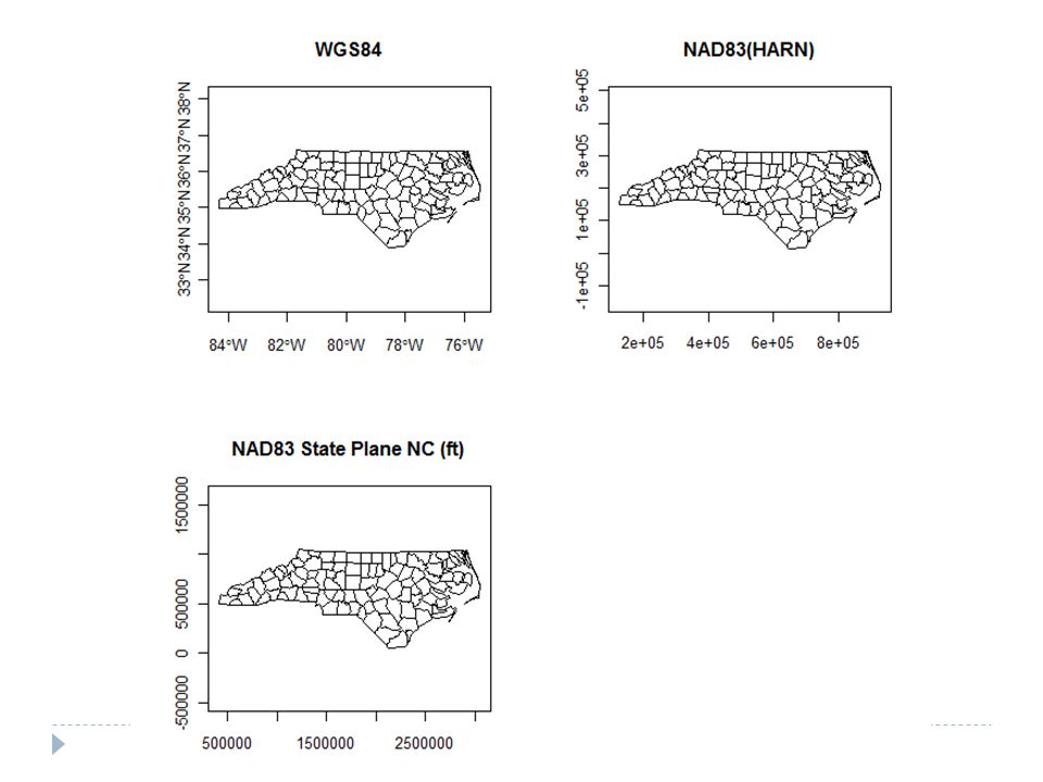
If the shapefile has no .prj file associated with it, you need to assign a coordinate system > proj4string(sids)<-CRS("+proj=longlat ellps=WGS84") We can then transform the map into any projection > sids_NAD<-spTransform(sids, CRS("+init=epsg:3358")) > sids_SP<-spTransform(sids, CRS("+init=ESRI:102719")) For a list of applicable CRS codes: Stick with the epsg and esri codes
<-CRS( +proj=longlat ellps=WGS84 ) We can then transform the map into any projection. > sids_NAD<-spTransform(sids, CRS( +init=epsg:3358 )) > sids_SP<-spTransform(sids, CRS( +init=ESRI: )) For a list of applicable CRS codes: Stick with the epsg and esri codes.")
14
Contiguity based neighbors
Areas sharing any boundary point (QUEEN) are taken as neighbors, using the poly2nb function, which accepts a SpatialPolygonsDataFrame > library(spdep) > sids_nbq<-poly2nb(sids) If contiguity is defined as areas sharing more than one boundary point (ROOK), the queen= argument is set to FALSE > sids_nbr<-poly2nb(sids, queen=FALSE) > coords<-coordinates(sids) > plot(sids) > plot(sids_nbq, coords, add=T)
 are taken as neighbors, using the poly2nb function, which accepts a SpatialPolygonsDataFrame. > library(spdep) > sids_nbq<-poly2nb(sids) If contiguity is defined as areas sharing more than one boundary point (ROOK), the queen= argument is set to FALSE. > sids_nbr<-poly2nb(sids, queen=FALSE) > coords<-coordinates(sids) > plot(sids) > plot(sids_nbq, coords, add=T)")
15
Queen Rook

16
Distance based neighbors k nearest neighbors
Can also choose the k nearest points as neighbors > coords<-coordinates(sids_SP) > IDs<-row.names(as(sids_SP, "data.frame")) > sids_kn1<-knn2nb(knearneigh(coords, k=1), row.names=IDs) > sids_kn2<-knn2nb(knearneigh(coords, k=2), row.names=IDs) > sids_kn4<-knn2nb(knearneigh(coords, k=4), row.names=IDs) > plot(sids_SP) > plot(sids_kn2, coords, add=T) k=1 k=2 k=3
 > IDs<-row.names(as(sids_SP, data.frame )) > sids_kn1<-knn2nb(knearneigh(coords, k=1), row.names=IDs) > sids_kn2<-knn2nb(knearneigh(coords, k=2), row.names=IDs) > sids_kn4<-knn2nb(knearneigh(coords, k=4), row.names=IDs) > plot(sids_SP) > plot(sids_kn2, coords, add=T) k=1. k=2. k=3.")
17
k=1 k=2 k=4

18
Distance based neighbors Specified distance
Can also assign neighbors based on a specified distance > dist<-unlist(nbdists(sids_kn1, coords)) > summary(dist) Min. 1st Qu. Median Mean 3rd Qu. Max. > max_k1<-max(dist) > sids_kd1<-dnearneigh(coords, d1=0, d2=0.75*max_k1, row.names=IDs) > sids_kd2<-dnearneigh(coords, d1=0, d2=1*max_k1, row.names=IDs) > sids_kd3<-dnearneigh(coords, d1=0, d2=1.5*max_k1, row.names=IDs) OR by raw distance > sids_ran1<-dnearneigh(coords, d1=0, d2=134600, row.names=IDs)
) > summary(dist) Min. 1st Qu. Median Mean 3rd Qu. Max > max_k1<-max(dist) > sids_kd1<-dnearneigh(coords, d1=0, d2=0.75*max_k1, row.names=IDs) > sids_kd2<-dnearneigh(coords, d1=0, d2=1*max_k1, row.names=IDs) > sids_kd3<-dnearneigh(coords, d1=0, d2=1.5*max_k1, row.names=IDs) OR by raw distance. > sids_ran1<-dnearneigh(coords, d1=0, d2=134600, row.names=IDs)")
19
dist=0.75*max_k1 (k=1) dist=1*max_k1=134600 dist=1.5*max_k1 dist=1*max_k1 dist=1.5*max_k1
 dist=1*max_k1= dist=1.5*max_k1 dist=1*max_k1 dist=1.5*max_k1")
20
Step 2: Assign weights to the areas that are linked
Creating spatial weights matrices using neighborhood lists

21
Spatial weights matrices
Once our list of neighbors has been created, we assign spatial weights to each relationship Can be binary or variable Even when the values are binary 0/1, the issue of what to do with no-neighbor observations arises Binary weighting will, for a target feature, assign a value of 1 to neighboring features and 0 to all other features Used with fixed distance, k nearest neighbors, and contiguity

22
Row-standardized weights matrix
> sids_nbq_w<- nb2listw(sids_nbq) > sids_nbq_w Characteristics of weights list: Neighbour list object: Number of regions: 100 Number of nonzero links: 490 Percentage nonzero weights: 4.9 Average number of links: 4.9 Weights style: W Weights constants summary: n nn S S S2 W Row standardization is used to create proportional weights in cases where features have an unequal number of neighbors Divide each neighbor weight for a feature by the sum of all neighbor weights Obs i has 3 neighbors, each has a weight of 1/3 Obs j has 2 neighbors, each has a weight of 1/2 Use is you want comparable spatial parameters across different data sets with different connectivity structures
 > sids_nbq_w. Characteristics of weights list: Neighbour list object: Number of regions: 100. Number of nonzero links: 490. Percentage nonzero weights: 4.9. Average number of links: 4.9. Weights style: W. Weights constants summary: n nn S0 S1 S2. W Row standardization is used to create proportional weights in cases where features have an unequal number of neighbors. Divide each neighbor weight for a feature by the sum of all neighbor weights. Obs i has 3 neighbors, each has a weight of 1/3. Obs j has 2 neighbors, each has a weight of 1/2. Use is you want comparable spatial parameters across different data sets with different connectivity structures.")
23
Binary weights > sids_nbq_wb<- nb2listw(sids_nbq, style="B") > sids_nbq_wb Characteristics of weights list: Neighbour list object: Number of regions: 100 Number of nonzero links: 490 Percentage nonzero weights: 4.9 Average number of links: 4.9 Weights style: B Weights constants summary: n nn S0 S1 S2 B Row-standardised weights increase the influence of links from observations with few neighbours Binary weights vary the influence of observations Those with many neighbours are up-weighted compared to those with few
 > sids_nbq_wb Characteristics of weights list: Neighbour list object: Number of regions: 100 Number of nonzero links: 490 Percentage nonzero weights: 4.9 Average number of links: 4.9 Weights style: B Weights constants summary: n nn S0 S1 S2 B Row-standardised weights increase the influence of links from observations with few neighbours. Binary weights vary the influence of observations. Those with many neighbours are up-weighted compared to those with few.")
24
Binary vs. row-standardized
A binary weights matrix looks like: A row-standardized matrix it looks like: 1 1 .5 .33

25
Regions with no neighbors
If you ever get the following error: Error in nb2listw(filename): Empty neighbor sets found You have some regions that have NO neighbors This is most likely an artifact of your GIS data (digitizing errors, slivers, etc), which you should fix in a GIS Also could have “true” islands (e.g., Hawaii, San Juans in WA) May want to use k nearest neighbors Or add zero.policy=T to the nb2listw call > sids_nbq_w<-nb2listw(sids_nbq, zero.policy=T)
: Empty neighbor sets found. You have some regions that have NO neighbors. This is most likely an artifact of your GIS data (digitizing errors, slivers, etc), which you should fix in a GIS. Also could have true islands (e.g., Hawaii, San Juans in WA) May want to use k nearest neighbors. Or add zero.policy=T to the nb2listw call. > sids_nbq_w<-nb2listw(sids_nbq, zero.policy=T)")
26
Step 3: Examine spatial autocorrelation
Using spatial weights matrices, run statistical tests of spatial autocorrelation

27
Spatial autocorrelation
Test for the presence of spatial autocorrelation Global Moran’s I Geary’s C Local (LISA – Local Indicators of Spatial Autocorrelation) Local Moran’s I and Getis Gi* We’ll just focus on the “industry standard” – Moran’s I
 Local Moran’s I and Getis Gi* We’ll just focus on the industry standard – Moran’s I.")
28
Moran’s I in R “two.sided” → HA: I ≠ I0 “greater” → HA: I > I0
> moran.test(sids_NAD$SIDR79, listw=sids_nbq_w, alternative=“two.sided”) Moran's I test under randomisation data: sids_NAD$SIDR79 weights: sids_nbq_w Moran I statistic standard deviate = , p-value = alternative hypothesis: greater sample estimates: Moran I statistic Expectation Variance “two.sided” → HA: I ≠ I0 “greater” → HA: I > I0 results reported here are actually for the default = “greater”
 Moran s I test under randomisation. data: sids_NAD$SIDR79. weights: sids_nbq_w. Moran I statistic standard deviate = , p-value = alternative hypothesis: greater. sample estimates: Moran I statistic Expectation Variance two.sided → HA: I ≠ I0. greater → HA: I > I0. results reported here are actually for the default = greater")
29
Moran’s I in R > moran.test(sids_NAD$SIDR79, listw=sids_nbq_wb)
Moran's I test under randomisation data: sids_NAD$SIDR79 weights: sids_nbq_wb Moran I statistic standard deviate = , p-value = alternative hypothesis: greater sample estimates: Moran I statistic Expectation Variance

30
Moving on to spatial regression
Modeling data in R

31
Spatial autocorrelation in residuals Spatial error model
Incorporates spatial effects through error term Where: If there is no spatial correlation between the errors, then = 0

32
Spatial autocorrelation in DV Spatial lag model
Incorporates spatial effects by including a spatially lagged dependent variable as an additional predictor Where: If there is no spatial dependence, and y does no depend on neighboring y values, = 0

33
Spatial Regression in R Example: Housing Prices in Boston
CRIM per capita crime rate by town ZN proportion of residential land zoned for lots over 25,000 ft2 INDUS proportion of non-retail business acres per town CHAS Charles River dummy variable (=1 if tract bounds river; 0 otherwise) NOX Nitrogen oxide concentration (parts per 10 million) RM average number of rooms per dwelling AGE proportion of owner-occupied units built prior to 1940 DIS weighted distances to five Boston employment centres RAD index of accessibility to radial highways TAX full-value property-tax rate per $10,000 PTRATIO pupil-teacher ratio by town B 1000(Bk )2 where Bk is the proportion of blacks by town LSTAT % lower status of the population MEDV Median value of owner-occupied homes in $1000's
 NOX. Nitrogen oxide concentration (parts per 10 million) RM. average number of rooms per dwelling. AGE. proportion of owner-occupied units built prior to DIS. weighted distances to five Boston employment centres. RAD. index of accessibility to radial highways. TAX. full-value property-tax rate per $10,000. PTRATIO. pupil-teacher ratio by town. B. 1000(Bk )2 where Bk is the proportion of blacks by town. LSTAT. % lower status of the population. MEDV. Median value of owner-occupied homes in $1000 s.")
34
Spatial Regression in R
Read in boston.shp Define neighbors (k nearest w/point data) Create weights matrix Moran’s test of DV, Moran scatterplot Run OLS regression Check residuals for spatial dependence Determine which SR model to use w/LM tests Run spatial regression model
 Create weights matrix. Moran’s test of DV, Moran scatterplot. Run OLS regression. Check residuals for spatial dependence. Determine which SR model to use w/LM tests. Run spatial regression model.")
35
Define neighbors and create weights matrix
> boston<-readOGR(dsn="F:/R/shapefiles",layer="boston") > class(boston) > boston$LOGMEDV<-log(boston$CMEDV) > coords<-coordinates(boston) > IDs<-row.names(as(boston, "data.frame")) > bost_kd1<-dnearneigh(coords, d1=0, d2=3.973, row.names=IDs) > plot(boston) > plot(bost_kd1, coords, add=T) > bost_kd1_w<- nb2listw(bost_kd1)
 > class(boston) > boston$LOGMEDV<-log(boston$CMEDV) > coords<-coordinates(boston) > IDs<-row.names(as(boston, data.frame )) > bost_kd1<-dnearneigh(coords, d1=0, d2=3.973, row.names=IDs) > plot(boston) > plot(bost_kd1, coords, add=T) > bost_kd1_w<- nb2listw(bost_kd1)")
36
Moran’s I on the DV > moran.test(boston$LOGMEDV, listw=bost_kd1_w)
Moran's I test under randomisation data: boston$LOGMEDV weights: bost_kd1_w Moran I statistic standard deviate = , p-value < 2.2e-16 alternative hypothesis: greater sample estimates: Moran I statistic Expectation Variance

37
Moran Plot for the DV > moran.plot(boston$LOGMEDV, bost_kd1_w, labels=as.character(boston$ID))
)")
38
OLS Regression bostlm<-lm(LOGMEDV~RM + LSTAT + CRIM + ZN + CHAS + DIS, data=boston) Residuals: Min 1Q Median 3Q Max Coefficients: Estimate Std. Error t value Pr(>|t|) (Intercept) < 2e-16 *** RM e-11 *** LSTAT < 2e-16 *** CRIM < 2e-16 *** ZN *** CHAS *** DIS e-06 *** --- Residual standard error: on 499 degrees of freedom Multiple R-squared: , Adjusted R-squared: F-statistic: on 6 and 499 DF, p-value: < 2.2e-16
 Residuals: Min 1Q Median 3Q Max Coefficients: Estimate Std. Error t value Pr(>|t|) (Intercept) < 2e-16 *** RM e-11 *** LSTAT < 2e-16 *** CRIM < 2e-16 *** ZN *** CHAS *** DIS e-06 *** --- Residual standard error: on 499 degrees of freedom Multiple R-squared: , Adjusted R-squared: F-statistic: on 6 and 499 DF, p-value: < 2.2e-16")
39
Checking residuals for spatial autocorrelation
> boston$lmresid<-residuals(bostlm) > lm.morantest(bostlm, bost_kd1_w) Global Moran's I for regression residuals Moran I statistic standard deviate = , p-value = 2.396e-09 alternative hypothesis: greater sample estimates: Observed Moran's I Expectation Variance
 > lm.morantest(bostlm, bost_kd1_w) Global Moran s I for regression residuals Moran I statistic standard deviate = , p-value = 2.396e-09 alternative hypothesis: greater sample estimates: Observed Moran s I Expectation Variance")
40
Determining the type of dependence
> lm.LMtests(bostlm, bost_kd1_w, test="all") Lagrange multiplier diagnostics for spatial dependence LMerr = , df = 1, p-value = 3.201e-07 LMlag = , df = 1, p-value = 8.175e-12 RLMerr = , df = 1, p-value = RLMlag = , df = 1, p-value = 4.096e-07 SARMA = , df = 2, p-value = 5.723e-12 Robust tests used to find a proper alternative Only use robust forms when BOTH LMErr and LMLag are significant There are 6 tests performed to assess the spatial dependence of the model. First, Moran’s I is .07, but highly significant (p<0.0001), indicating strong spatial autocorrelation in the residuals. There are also 5 LM tests: The LM test for a missing spatially lagged DV (LMlag) The LM test for error dependence (LMerr) The robust LM error, which tests for error dependence in the possible presence of a missing lagged dependent variable The robust LM lag, which tests for The SARMA test, which tests for both lag and error (not particularly useful because it’s high if either SL or SE is present) We see that both simple LM tests are significant, indicating the presence of spatial dependence The robust tests help us understand what type of spatial dependence may be at work…both are significant, but the lag measures is more so. This tells us we should run a spatial lag model.
 Lagrange multiplier diagnostics for spatial dependence. LMerr = , df = 1, p-value = 3.201e-07. LMlag = , df = 1, p-value = 8.175e-12. RLMerr = , df = 1, p-value = RLMlag = , df = 1, p-value = 4.096e-07. SARMA = , df = 2, p-value = 5.723e-12. Robust tests used to find a proper alternative. Only use robust forms when BOTH LMErr and LMLag are significant. There are 6 tests performed to assess the spatial dependence of the model. First, Moran’s I is .07, but highly significant (p<0.0001), indicating strong spatial autocorrelation in the residuals. There are also 5 LM tests: The LM test for a missing spatially lagged DV (LMlag) The LM test for error dependence (LMerr) The robust LM error, which tests for error dependence in the possible presence of a missing lagged dependent variable. The robust LM lag, which tests for. The SARMA test, which tests for both lag and error (not particularly useful because it’s high if either SL or SE is present) We see that both simple LM tests are significant, indicating the presence of spatial dependence. The robust tests help us understand what type of spatial dependence may be at work…both are significant, but the lag measures is more so. This tells us we should run a spatial lag model.")
41
One more diagnostic… Indicates errors are heteroskedastic
> install.packages(“lmtest”) > library(lmtest) > bptest(bostlm) studentized Breusch-Pagan test data: bostlm BP = , df = 6, p-value = 2.651e-13 Indicates errors are heteroskedastic Not surprising since we have spatial dependence
 > library(lmtest) > bptest(bostlm) studentized Breusch-Pagan test. data: bostlm. BP = , df = 6, p-value = 2.651e-13. Indicates errors are heteroskedastic. Not surprising since we have spatial dependence.")
42
Running a spatial lag model
> bostlag<-lagsarlm(LOGMEDV~RM + LSTAT + CRIM + ZN + CHAS + DIS, data=boston, bost_kd1_w) Type: lag Coefficients: (asymptotic standard errors) Estimate Std. Error z value Pr(>|z|) (Intercept) < 2.2e-16 RM e-10 LSTAT < 2.2e-16 CRIM < 2.2e-16 ZN CHAS DIS e-11 Rho: , LR test value:37.426, p-value:9.4936e-10 Asymptotic standard error: z-value: , p-value: e-11 Wald statistic: , p-value: e-11 Log likelihood: for lag model ML residual variance (sigma squared): , (sigma: ) AIC: , (AIC for lm: ) Rho reflects the spatial dependence inherent in our sample data, measuring the average influence on observations by their neighboring observations. It has a positive effect and is highly significant. AIC is lower that linear model, indicating a better model fit. However, the LR test value (likelihood ratio) is still significant, indicating that the introduction of the spatial lag term improved model fit, it didn’t make the spatial effects go away.
 Type: lag Coefficients: (asymptotic standard errors) Estimate Std. Error z value Pr(>|z|) (Intercept) < 2.2e-16 RM e-10 LSTAT < 2.2e-16 CRIM < 2.2e-16 ZN CHAS DIS e-11 Rho: , LR test value:37.426, p-value:9.4936e-10 Asymptotic standard error: z-value: , p-value: e-11 Wald statistic: , p-value: e-11 Log likelihood: for lag model ML residual variance (sigma squared): , (sigma: ) AIC: , (AIC for lm: ) Rho reflects the spatial dependence inherent in our sample data, measuring the average influence on observations by their neighboring observations. It has a positive effect and is highly significant. AIC is lower that linear model, indicating a better model fit. However, the LR test value (likelihood ratio) is still significant, indicating that the introduction of the spatial lag term improved model fit, it didn’t make the spatial effects go away.")
43
A few more diagnostics LM test for residual autocorrelation test value: , p-value: > bptest.sarlm(bostlag) studentized Breusch-Pagan test data: BP = , df = 6, p-value = 4.451e-11 LM test suggests there is no more spatial autocorrelation in the data BP test indicates remaining heteroskedasticity in the residuals Most likely due to misspecification
 studentized Breusch-Pagan test. data: BP = , df = 6, p-value = 4.451e-11. LM test suggests there is no more spatial autocorrelation in the data. BP test indicates remaining heteroskedasticity in the residuals. Most likely due to misspecification.")
44
Running a spatial error model
> bosterr<-errorsarlm(LOGMEDV~RM + LSTAT + CRIM + ZN + CHAS + DIS, data=boston, listw=bost_kd1_w) Type: error Coefficients: (asymptotic standard errors) Estimate Std. Error z value Pr(>|z|) (Intercept) < 2.2e-16 RM e-09 LSTAT < 2.2e-16 CRIM < 2.2e-16 ZN CHAS DIS Lambda: , LR test value: , p-value: e-07 Asymptotic standard error: z-value: , p-value: e-12 Wald statistic: 46.35, p-value: e-12 Log likelihood: for error model ML residual variance (sigma squared): , (sigma: ) AIC: , (AIC for lm: )
 Type: error Coefficients: (asymptotic standard errors) Estimate Std. Error z value Pr(>|z|) (Intercept) < 2.2e-16 RM e-09 LSTAT < 2.2e-16 CRIM < 2.2e-16 ZN CHAS DIS Lambda: , LR test value: , p-value: e-07 Asymptotic standard error: z-value: , p-value: e-12 Wald statistic: 46.35, p-value: e-12 Log likelihood: for error model ML residual variance (sigma squared): , (sigma: ) AIC: , (AIC for lm: )")
Similar presentations