Download presentation
Presentation is loading. Please wait.

1
2-5 : Normal Distribution

2
Standard Deviation Calculate the mean Given a Data Set 12, 8, 7, 14, 4
= 9 The standard deviation is a measure of the mean spread of the data from the mean. How far is each data value from the mean? ( ) ÷ 5 = 12.8 Square to remove the negatives Square root 12.8 = 3.58 25 1 9 4 Std Dev = 3.58 4 7 14 12 8 -2 -1 3 5 -5 Average = Sum divided by how many values Calculator function Square root to ‘undo’ the squared
 ÷ 5 = Square to remove the negatives. Square root 12.8 = Std Dev = Average = Sum divided by how many values. Calculator function. Square root to ‘undo’ the squared.")
3
NORMAL DISTRIBUTIONS : Vocabulary
Normal curves are used in many situations to estimate probabilities. The pattern the data form is a bell-shaped curve called a normal curve. NORMAL DISTRIBUTION ̶ shows data that vary randomly from the mean in the pattern of a bell-shaped curve.

4
NORMAL DISTRIBUTIONS : Vocabulary
1. Maximum value of the curve occurs at the mean, usually symbolized as 𝜇, (Greek letter mu). 2. The standard deviation of 𝜎(sigma). 3. Nearly all of the area under the curve (99.7%) is within three standard deviations from the mean, 𝜇±3𝜎 4. The total area under a normal curve is always The area under the curve between two x-values corresponds to the probability that x is between those values.
. 2. The standard deviation of 𝜎(sigma). 3. Nearly all of the area under the curve (99.7%) is within three standard deviations from the mean, 𝜇±3𝜎 4. The total area under a normal curve is always The area under the curve between two x-values corresponds to the probability that x is between those values.")
5
Properties of Normal Distributions
μ 3σ μ + σ μ 2σ μ σ μ μ + 2σ μ + 3σ Total area = 1 x If x is a continuous random variable having a normal distribution with mean μ and standard deviation σ.

6
The Standard Normal Distribution
The standard normal distribution is a normal distribution with a mean of 0 and a standard deviation of 1. The horizontal scale corresponds to z-scores. z 3 2 1 1 2 3 Any value can be transformed into a z-score by using the formula

7
The Standard Normal Table
Properties of the Standard Normal Distribution The cumulative area is close to 0 for z-scores close to z = 3.49. The cumulative area increases as the z-scores increase. The cumulative area for z = 0 is The cumulative area is close to 1 for z-scores close to z = 3.49 z 3 1 2 1 2 3 z = 3.49 Area is close to 1. z = 0 Area is z = 3.49 Area is close to 0.

8
Z-Scores EX #7: Use the data from EX #4. Plot the data values and the mean on the line plot. Do all of the values fall between two standard deviations of mean? No : 32 MWH is more than 2 standard deviation below the mean. B. In August, the mean daily energy requirements is 39.4 MWh, with a standard deviation of 3.2 MWh. The power company makes plans for any demand within three standard deviations of the mean. Will they be prepared for a demand of 51 MWh? Explain. 𝑥 +3𝜎 (3.2) = 49 ; No, 51 is an outlier. C. Find the z-score. 𝑧= 61− = 2.7
 = 49 ; No, 51 is an outlier. C. Find the z-score. 𝑧= 61−45 6 = 2.7.")
9
Estimating Probabilities Using A Normal Curve
EX #1: In a survey of American men, the heights are distributed normally about the mean, as shown in the graph above. About what percent of men aged 26 to 35 are 68 – 70 inches tall? ≈ 40.2% B. About what percent of the men in the survey are less than 70 inches tall? ≈ 40% C. Suppose this survey was the data on 1500 men. About how many men would you expect to be 68 – 70 inches tall? (0.402)(1500) ≈603 𝑚𝑒𝑛 D. The mean of the data is 70, and the standard deviation is 2.5. About what percent of the men are within one standard deviation of the mean in height? = 67.5 = 72.5 ≈ 66.4%
(1500) ≈603 𝑚𝑒𝑛. D. The mean of the data is 70, and the standard deviation is 2.5. About what percent of the men are within one standard deviation of the mean in height = = ≈ 66.4%")
10
Sketching a Normal Curve
EX #2: The table below shows the lengths, in feet, of 40 great white sharks from Scuba News Magazine. A. Enter these data items into your calculator and make a histogram B. Calculate one-variable statistics.

11
Sketching a Normal Curve
C. Sketch a normal curve, showing the frequency of the shark lengths. Label the x-axis values at one, two, and three standard deviations from the mean. μ 3σ 8.2 μ + σ 18.2 μ 2σ 10.7 μ σ 13.2 μ 15.7 μ + 2σ 20.7 μ + 3σ 23.2 Total area = 1 x 12 12 4 5 1 1

12
The Normal Distribution
Key Concepts Area under the graph is the relative frequency = the probability Total Area = 1 The MEAN is in the middle. The distribution is symmetrical. 1 Std Dev either side of mean = 68% A lower mean A higher mean 2 Std Dev either side of mean = 95% 3 Std Dev either side of mean = 99% A smaller Std Dev. A larger Std Dev. Distributions with different spreads have different STANDARD DEVIATIONS

13
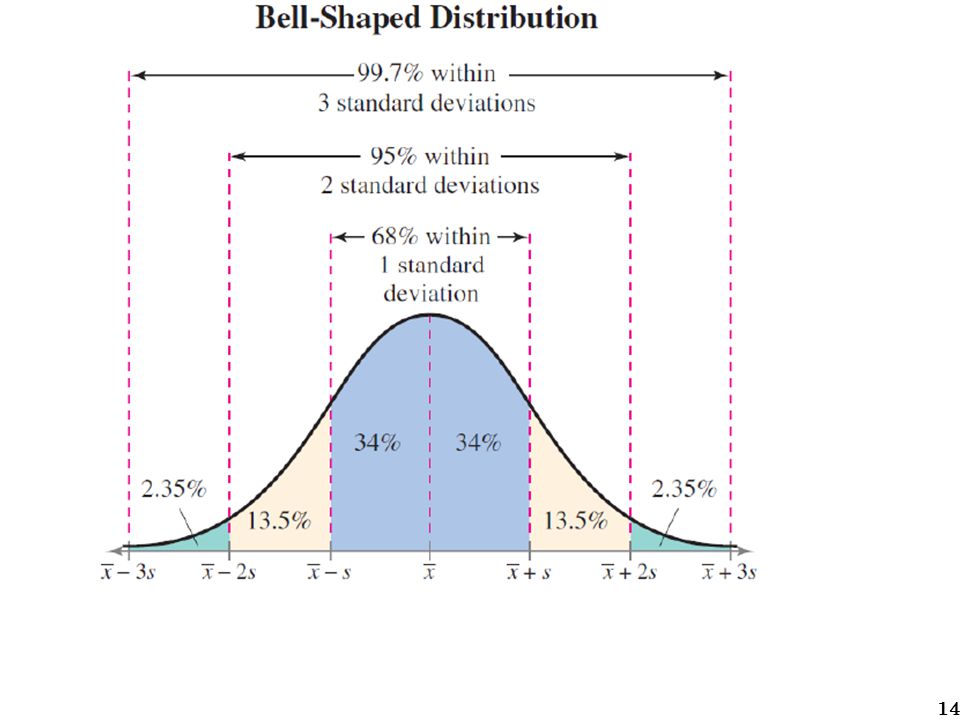
The 68 – 95 – 99.7 Rule When a data set is normally distributed, about 68% of the data fall within one standard deviation of the mean. About 95% of the data fall within two standard deviations of the mean. In order to find the values that are two standard deviations away from the mean, we would find the values that have a z-score of ±2. Sometimes called The Empirical Rule: The 68 – 95– 99.7 Rule In a Normal distribution with mean 𝜇 and standard deviation 𝜎: • Approximately 68% of the observations fall within 𝜎 of the mean. • Approximately 95% of the observations fall within 2𝜎 of the mean. • Approximately 99.7% of the observations fall within 3𝜎 of the

15
Using Standard Normal Values
If a random variable x is normally distributed with mean 𝜇 and standard deviation 𝜎𝜎, then the standard normal value of x is 𝑧= 𝑥 −𝜇 𝜎 The table shows the approximate area under the curve for all values less than z for selected values of z. EX #3: Scores on a test are normally distributed with a mean of 76 and a standard deviation of 8. A. Estimate the probability that a randomly selected student scored less than 88%. 𝑧= 88−76 8 = 1.5 Find area under the curve for all values less than 1.5 or about 0.93 ∴𝑃𝑟𝑜𝑏𝑎𝑏𝑖𝑙𝑖𝑡𝑦 𝑜𝑓 𝑠𝑐𝑜𝑟𝑖𝑛𝑔 𝑎𝑛 88 𝑖𝑠 𝑎𝑏𝑜𝑢𝑡 93 %

16
Using Standard Normal Values
B. Estimate the probability that a randomly selected student scored between 72 and 80. 𝑧 2 = 80−76 8 𝑧 2 = 0.5 𝑧 1 = 72−76 8 𝑧 1 = -0.5 Area ≈0.31 Area ≈0.69 Since these area overlap subtract = 0.38 ∴𝑃𝑟𝑜𝑏𝑎𝑏𝑖𝑙𝑖𝑡𝑦 𝑜𝑓 𝑠𝑐𝑜𝑟𝑖𝑛𝑔 𝑏𝑒𝑡𝑤𝑒𝑒𝑛 72 𝑎𝑛𝑑 80 𝑖𝑠 𝑎𝑏𝑜𝑢𝑡 38% μ 3σ μ + σ μ 2σ μ σ μ μ + 2σ μ + 3σ Total area = 1 x

17
Skewness Negatively Skewed Positively Skewed Symmetric (Not Skewed)
")
18
Skewness Negatively Symmetric Positively Skewed (Not Skewed) Mean Mode
Median Mean Symmetric (Not Skewed) Positively
 Positively.")
19
Is It Normal or Skewed? While many data sets can be modeled using a normal curve, not all data is normally distributed. Sometimes the “tail” is longer on one side than the other, resulting in a skewed distribution.

20
Is It Normal or Skewed? EX #4: The heights of 24 children entering a theme park are shown below. The mean of all the children at the park is 49 inches and the standard deviation is 6 inches. A. Does the data appear to be normally distributed? Explain your reasoning. No, this data is skewed positively or left. There are more values above 49 inches than below.

21
Is It Normal or Skewed? B. Use your calculator to draw a histogram and calculate one-variable statistics.

22
Real-World Connection
EX #5: In a college algebra course with 286 students in a lecture hall, the final exam scores have a mean of 67.5 and a standard deviation of 7.4. The grades on the exams are all whole numbers, and the grade pattern follows a normal curve. A. Sketch a normal curve, label the x-axis values at one, two, and three standard deviations from the mean. μ 3σ = 45.3 μ + σ = 74.9 μ 2σ = 52.7 μ= 67.5 μ + 2σ = 89.7 μ + 3σ Total area = 1 x 97 97 39 39 7 7 μ σ = 60.1

23
Real-World Connection
B. Find the number of students who receive grades from one to two standard deviations above the mean. 0.135(285) = ≈38 𝑜𝑟 39 𝑠𝑡𝑢𝑑𝑒𝑛𝑡𝑠 C. How many students earned a grade below 60%? 13.5% +2.5% = 16% 0.16(286) = 4.76 About 46 students earned 60 or below. D. Suppose the class only had 170 students. About how many students would earn a grade of 82 or more? 0.16(170) = 27.2 ≈27 𝑠𝑡𝑢𝑑𝑒𝑛𝑡𝑠
 = ≈38 𝑜𝑟 39 𝑠𝑡𝑢𝑑𝑒𝑛𝑡𝑠. C. How many students earned a grade below 60% 13.5% +2.5% = 16% 0.16(286) = About 46 students earned 60 or below. D. Suppose the class only had 170 students. About how many students would earn a grade of 82 or more 0.16(170) = 27.2 ≈27 𝑠𝑡𝑢𝑑𝑒𝑛𝑡𝑠.")
24
Find the probability a chicken is less than 4kg
Finding a Probability 1st slide The mean weight of a chicken is 3 kg (with a standard deviation of 0.4 kg) Find the probability a chicken is less than 4kg 4kg 3kg Draw a distribution graph 1 How many Std Dev from the mean? 4kg distance from mean standard deviation = = 2.5 1 0.4 3kg Look up 2.5 Std Dev in tables (z = 2.5) 0.5 0.4938 Probability = (table value) = 4kg 3kg So 99.38% of chickens in the population weigh less than 4kg
 Find the probability a chicken is less than 4kg. 4kg. 3kg. Draw a distribution graph. 1. How many Std Dev from the mean 4kg. distance from mean. standard deviation. = = kg. Look up 2.5 Std Dev in tables (z = 2.5) Probability = (table value) = kg. 3kg. So 99.38% of chickens in the population weigh less than 4kg.")
25
Standard Normal Distribution
1st slide The mean weight of a chicken is 2.6 kg (with a standard deviation of 0.3 kg) Find the probability a chicken is less than 3kg 3kg 2.6kg Draw a distribution graph Table value 0.5 Change the distribution to a Standard Normal distance from mean standard deviation z = = = 1.333 0.4 0.3 z = 1.333 Aim: Correct Working The Question: P(x < 3kg) = P(z < 1.333) Look up z = Std Dev in tables = Z = ‘the number of standard deviations from the mean’ =
 Find the probability a chicken is less than 3kg. 3kg. 2.6kg. Draw a distribution graph. Table value Change the distribution to a Standard Normal. distance from mean. standard deviation. z = = = z. = Aim: Correct Working. The Question: P(x < 3kg) = P(z < 1.333) Look up z = Std Dev in tables. = Z = ‘the number of standard deviations from the mean’ =")
26
Inverse Normal Distribution
1st slide The mean weight of a chicken is 2.6 kg (with a standard deviation of 0.3 kg) 2.6kg ‘x’ kg Area = 0.9 90% of chickens weigh less than what weight? (Find ‘x’) Draw a distribution graph 0.4 0.5 Look up the probability in the middle of the tables to find the closest ‘z’ value. Z = ‘the number of standard deviations from the mean’ z = 1.281 The closest probability is Look up 0.400 Corresponding ‘z’ value is: 1.281 z = 1.281 2.6kg D D = × 0.3 The distance from the mean = ‘Z’ × Std Dev 2.98 kg x = 2.6kg = kg
 2.6kg. ‘x’ kg. Area = % of chickens weigh less than what weight (Find ‘x’) Draw a distribution graph Look up the probability in the middle of the tables to find the closest ‘z’ value. Z = ‘the number of standard deviations from the mean’ z. = The closest probability is Look up Corresponding ‘z’ value is: z = kg. D. D = × 0.3. The distance from the mean = ‘Z’ × Std Dev kg. x = 2.6kg = kg.")
Similar presentations