1. Effect Modification & Confounding
Kostas Danis
EPIET Introductory course,
Menorca 2012
Lecture notes

2. Analytical epidemiology
Study design: cohorts & case control &
cross-sectional studies
Choice of a reference group
Biases
Impact
Causal inference
Stratification
- Effect modification - Confounding
Matching
Multivariable analysis

3. Cohort studies marching towards outcomes

4. Cohort study Non cases Risk % Total Cases Exposed 100 50 50 50 %%
Not exposed
100 %
Risk ratio % / 10% = 5

5. Cases Controls Source population Exposed Sample Unexposed Controls:
Sample of the denominator
Representative with
regard to exposure
Controls

6. Controls are non cases
Cases
Source popn
Low attack rate: non-cases likely to represent exposure in source pop
Non- cases
start
end
High attack rate: non-cases unlikely to represent exposure in source population
Cases
Non- cases
start
end

7. a/c b/d Case control study Cases Controls Odds ratio a b Exposed
OR= (a/c) / (b/d)
= ad / bc
Not exposed
c d
a+c
Total
b+d
Odds of
exposure
a/c
b/d

8. Who are the right controls?
If we are able of defining the population source of our cases, we still have to decide which one we will choose as a control.

9. Controls may not be easy to find
Usually it is more complicated to find a control than a case in birds and in humans.

10. Cross-sectional study: Sampling
Sample
Sampling
Population
When we want to take a sample we first need to define our target population. The target population is the population about which you want information, that you wish to make conclusions about from the results of the study. The study or sampling population is the population from which the sample (sampling frame) is drawn (the population from which you select your sample). It may be a more limited, an accessible population. For example, suppose you want to estimate the prevalence of flu-like symptoms in a country and you conduct telephone interviews; Your target population will be the total population in the country and the study population will be all people with telephones. Or if you want to estimate the vaccination coverage among 6 year old children in Spain and you take a sample of school children; your target population is all 6 year olds in Spain, whereas your sampling population is all first Grammar class school children.
Target Population

11. Cross-sectional study
Non
cases Prevalence %
Total
Cases
Exposed
1,000 %
Not exposed
1,000 %
Prevalence ratio (PR) % / 10% = 5

12. Should I believe my measurement?
Exposure Outcome
RR = 4
True association
causal
non-causal
Chance?
Bias?
Confounding?

13. Exposure Outcome
Third variable

14. Two main complications
(1) Effect modifier
(2) Confounding factor
- useful information
- bias

15. To analyse effect modification
To eliminate confounding
Solution = stratification
stratified analysis
Create strata
according to categories
inside the range of values
taken by third variable

16. Effect modification

17. Effect modifier
Variation in the magnitude of measure of effect across levels of a third variable.
Happens when RR or OR is different between strata (subgroups of population)

18. Effect modifier
To identify a subgroup with a lower or higher risk ratio
To target public health action
To study interaction between risk factors

19. Effect modification Disease Factor A (lung cancer) (asbestos) Factor B
(smoking)
Effect modifier = Interaction

20. Asbestos (As) and lung cancer (Ca)
Case-control study, unstratified data
As Ca Controls OR
Yes
No Ref.
Total

21. Asbestos Lung cancer
Smoking

23. Asbestos (As), smoking and lung cancer (Ca)
As Smoking Cases Controls OR
Yes Yes
Yes No
No Yes
No No Ref.
1.5 * 3.0 < * 3.0 * interaction=8.9

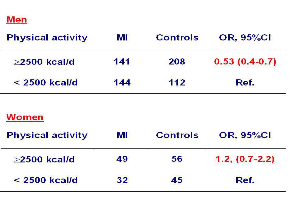
24. Physical activity and MI

25. Physical Infarction activity
Gender

27. Vaccine efficacy
ARU – ARV
VE =
ARU
VE = 1 – RR

28. Vaccine efficacy
VE = RR =
VE = 72%

29. Vaccine Disease
Age

30. Vaccine efficacy by age group

31. Effect modification
Different effects (RR) in different strata (age groups)
VE is modified by age
Test for homogeneity among strata (Woolf test)

32. Any statistical test to help us?
Breslow-Day
Woolf test
Test for trends: Chi square
Homogeneity

33. How to conduct a stratified analysis?
Crude analysis
Stratified analysis
Do stratum-specific estimates look different?
95% CI of OR/RR do NOT overlap?
Is the Test of Homogeneity significant? NO
Check for confounding
(compare crude RR/OR
with MH RR/OR)
YES
EFFECT MODIFICATION
(Report estimates by stratum)

34. Stratified analysis: Effect Modification

35. Death from diarrhea according to breast feeding, Brazil, 1980s (Crude analysis)
Diarrhea Controls OR (95% CI)
No breast feeding ( )
Breast feeding Ref

36. No breast Diarhoea
feeding
Age

37. Death from diarrhea according to breast feeding, Brazil, 1980s
Infants < 1 month of age
Cases Controls OR (95% CI)
No breast feeding (6-203)
Breast feeding Ref
Infants ≥ 1 month of age
Cases Controls OR (95% CI)
No breast feeding ( )
Breast feeding Ref
Woolf test (test of homogeneity):p=0.03

38. Risk of gastroenteritis by exposure, Outbreak X, Place, time X (crude analysis)
Exposed
Exposure
Yes No
RR†
(95% CI‡) n
AR (%)*
AR(%)*
pasta 94 77 7
4.2
18.0
(8.8-38)
tuna 49 68 24
2.9
( )
* AR = Attack Rate
† RR = Risk Ratio
‡ 95% CI = 95% confidence interval of the RR

39. Tuna gastroenteritis
Pasta

40. Risk of gastroenteritis by exposure, Outbreak X, Place, time X (stratified analysis)
Pasta Yes
Cases Total AR (%) RR (95% CI)
Tuna ( )
No tuna Ref
Pasta No
Cases Total AR (%) RR (95% CI) Tuna (2.6-46)
No tuna Ref
Woolf test (test of homogeneity): p=0.0007

41. Tuna, pasta and gastroenteritis
Tuna Pasta Cases AR(%) RR
Yes Yes
Yes No
No Yes
No No Ref.
38 * 12 > * 12 * interaction= 42

42. Risk of HIV by injecting drug use (idu), surveillance data, Spain, 1988-2004
Cases Total AR (%) RR (95% CI)
Idu , ( )
No idu , Ref

43. idu hiv
gender

44. Risk of HIV by injecting drug use (idu), Spain, 1988-2004 (stratified analysis)
Males
Cases Total AR (%) RR (95% CI)
idu (14-28)
No idu , Ref
Females
Cases Total AR (%) RR (95% CI) idu , ( )
No idu , Ref
Woolf test (test of homogeneity): p=

45. Idu, gender and hiv Idu Male Cases AR(%) RR Yes Yes 86 12.4 3.0
Yes No
No Yes
No No Ref.
0.14 * 2.2 > * 2.2 * interaction= 3.0

47. Confounding

48. Confounding Distortion of measure of effect because of a third factor
Should be prevented
Needs to be controlled for

49. Confounding Skate- boarding Chlamydia Age
Age not evenly distributed between the 2 exposure groups - skate-boarders, 90% young - Non skate-boarders, 20% young

50. Exposure Outcome
(coffee) (Lung cancer)
Third variable
(smoking)

51. Grey hair stroke
Age

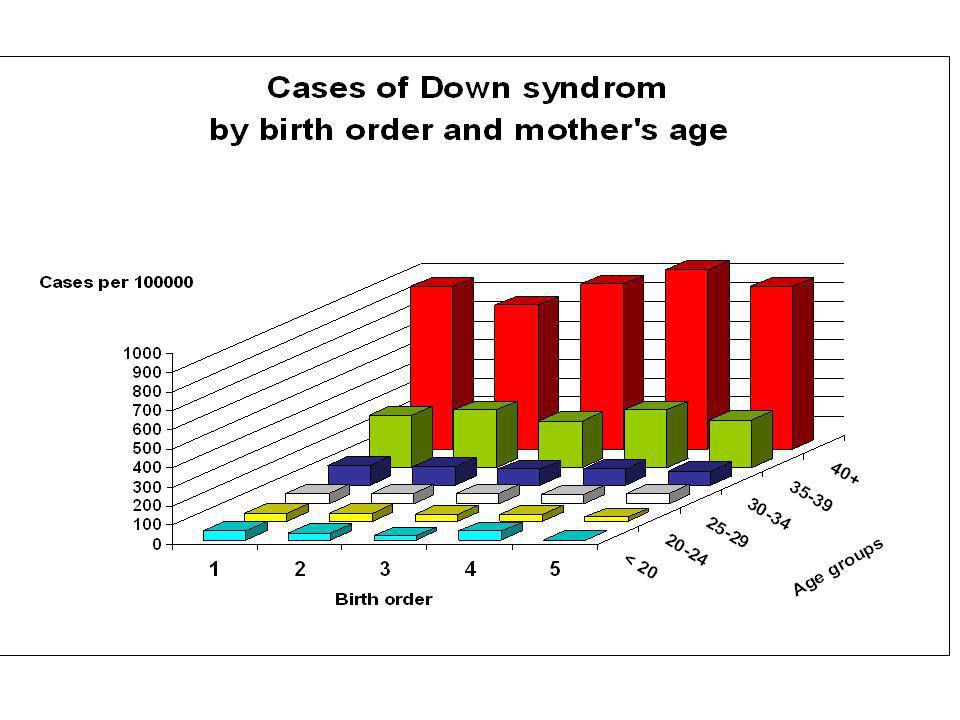
54. Birth
order
Down
syndrom
Age or
mother

56. Confounding Exposure Outcome Third variable
To be a confounding factor, 2 conditions must be met:
Exposure
Outcome
Third variable
Be associated with exposure
- without being the consequence of exposure
Be associated with outcome
- independently of exposure

57. Exposure Outcome Third factor
Hypercholesterolaemia Myocardial infarction
Third factor
Atheroma
Any factor which is a necessary step in the causal chain is not a confounder

58. Salt Myocardial infarction
Hypertension

59. The nuisance introduced by confounding factors
May simulate an association
May hide an association that does exist
May alter the strength of the association
Increased
Decreased
Confounding factor

60. Apparent association
Ethnicity Pneumonia
Crowding

61. Altered strength of association
Crowding Pneumonia
Malnutrition

62. How to prevent/control confounding?
Prevention
Randomization (experiment)
Restriction to one stratum
Matching
Control
Stratified analysis
Multivariable analysis

63. Are Mercedes more dangerous than Porsches?
95% CI =

64. Car type Accidents
Confounding factor:
Age of driver

65. Crude RR = 1.5
Adjusted RR = 1.1 ( )

66. Crude data Malaria Total AR% RR Radio set 80 520 15 0.7
Incidence of malaria according to the presence of a radio set, Kahinbhi Pradesh
Crude data Malaria Total AR% RR
Radio set
No radio Ref
RR: 0.7; 95% CI: ; p < 0.02
95% CI =

67. Radio Malaria
Confounding factor:
Mosquito net

68. Crude RR = 0.7
Adjusted RR = 1.01

69. To identify confounding
Compare crude measure of effect (RR or OR) to
adjusted (weighted) measure of effect
(Mantel Haenszel RR or OR)

70. Any statistical test to help us?
When is ORMH different from crude OR ? %

71. Mantel-Haenszel summary measure
Adjusted or weighted RR or OR
Advantages of MH
Zeroes allowed
S (ai di) / ni
OR MH =
S (bi ci) / ni

72. Mantel-Haenszel summary measure
Mantel-Haenszel (adjusted or weighted) OR a1 b1 c1 d1
Cases
Controls
Exp+
Exp-
OR MH =
SUM (ai di / ni)
SUM (bi ci / ni) n1
Cases
Controls
(a1 x d1) / n1 +
ORMH =
(a2 x d2) / n2
Exp+ a2 b2
(b1 x c1) / n1 +
(b2 x c2) / n2
Exp- d2 c2 n2

73. How to conduct a stratified analysis?
Crude analysis
Stratified analysis
Do stratum-specific estimates look different?
95% CI of OR/RR do NOT overlap?
Is the Test of Homogeneity significant? NO
Check for confounding
(compare crude RR/OR
with MH RR/OR)
YES
EFFECT MODIFICATION
(Report estimates by stratum)

74. Risk of gastroenteritis by exposure, Outbreak X, Place, time X (crude analysis)
???

75. Stratified Analysis
> 10-20%

76. Examples of stratified analysis

77. Weighted RR different from crude RR
Effect modifier
Belongs to nature
Different effects in different strata
Simple
Useful
Increases knowledge of biological mechanism
Allows targeting of PH action
Confounding factor
Belongs to study
Weighted RR different from crude RR
Distortion of effect
Creates confusion in data
Prevent (protocol)
Control (analysis)

78. Analyzing a third factor

79. How to conduct a stratified analysis
Perform crude analysis Measure the strength of association
List potential effect modifiers and confounders
Stratify data according to potential modifiers or confounders
Check for effect modification
If effect modification present, show the data by stratum
If no effect modification present, check for confounding If confounding, show adjusted data If no confounding, show crude data

80. How to define the strata?
Strata defined according to third variable:
‘Usual’ confounders (e.g. age, sex, socio-economic status)
Any other suspected confounder, effect modifier or additional risk factor
Stratum of public health interest
For two risk factors:
stratify on one to study the effect of the second on outcome
Two or more exposure categories:
each is a stratum
Residual confounding ?

81. Logical order of data analysis
How to deal with multiple risk factors:
Crude analysis
Multivariable analysis
1. stratified analysis
2. modelling
linear regression
logistic regression

82. Multivariate analysis
Mathematical model
Simultaneous adjustment of all confounding and risk factors
Can address effect modification

83. A train can mask a second train
A variable can mask another variable

85. Back-up slides

86. Risk factors for Salmonella enteritidis infections, France, 1995
Delarocque-Astagneau et al Epidemiol. Infect 1998:121:561-7

87. Cases of Salmonella enteritidis gastroenteritis according to egg storage and season
Summer
Cases
Controls OR
(95%CI)
Duration of storage
>= 2 weeks 12 2
7.4
( )
< 2 weeks 52 64
Other seasons 7 3
2.6
( ) 32 36
All seasons 19 5
4.5
(1.5 – 16.1) 84
100

88. Duration Salmonellosis
of storage
Season

89. Cases of Salmonella enteritidis gastroenteritis according to egg storage and season
Summer
(A)
“Long” storage
(B)
Cases
Control OR
Yes 12 2
ORAB
6.8 No 52 64
ORA
0.9 7 3
ORB
2.6 32 36
Ref

90. Advantages & Disadvantages of Stratified Analysis
straightforward to implement and comprehend
easy way to evaluate interaction
Disadvantages
only one exposure-disease association at a time
requires continuous variables to be grouped
Loss of information; possible “residual confounding”
deteriorates with multiple confounders
e.g. suppose 4 confounders with 3 levels
3x3x3x3=81 strata needed
unless huge sample, many cells have “0”’ and strata have undefined effect measures