Download presentation
Presentation is loading. Please wait.

1
Micro Design

5
System Capacity

6
Crop Water Needs Example Calculate capacity required for a proposed 1 ac. Micro irrigation system on Vegetables. Using drip tape with a flow of 0.45 gpm/100’ and 12” emitter spacing, 200 ft rows, 5 ft row spacing, and 10 fields of 0.1 ac each. Q = 453*DA T D =.2” / system efficiency A = Area T = 22 hrs

7
Crop Water Needs Example Answer Q = 453*DA T =453 x (.2”/.9) x 1 ac 22 hrs =4.5 gpm
 x 1 ac 22 hrs =4.5 gpm")
8
Each field will have a capacity of 4.5 gpm. ◦ 200 ft rows with a 0.45 gpm/100’ drip tape flow will give you 0.9 gpm per row. ◦ At 5 ft row spacing, 1 ac will have approximately 10 fields, each of these fields will have 5 rows, 200 ft long. ◦ 5 rows times 0.9 gpm/row is 4.5 gpm per field. Minimum water requirement is 4.5 gpm for 1 ac, we only need to run 1 field at a time to meet the crop water demand.

9
Hours of irrigation per day to apply.2” (1 field of 0.1 ac each) T = 453*DA Q =453 x (.2”/.9) x 0.1 ac 4.5 gpm =2 hrs and 15 minutes
 T = 453*DA Q =453 x (.2 /.9) x 0.1 ac 4.5 gpm =2 hrs and 15 minutes")
10
WELL 8:00 a.m. field 1 2 hrs and 15 min @ 4.5 gpm 10:15 a.m. field 2 2 hrs and 15 min @ 4.5 gpm 12:30 p.m. field 3 2 hrs and 15 min @ 4.5 gpm 2:45 p.m. field 4 2 hrs and 15 min @ 4.5 gpm 5:15 p.m. field 5 2 hrs and 15 min @ 4.5 gpm 7:30 p.m. field 6 2 hrs and 15 min @ 4.5 gpm 9:45 p.m. field 7 2 hrs and 15 min @ 4.5 gpm 12:00 a.m. field 8 2 hrs and 15 min @ 4.5 gpm 2:15 a.m. field 9 2 hrs and 15 min @ 4.5 gpm 4:30 a.m. field 10 2 hrs and 15 min @ 4.5 gpm

11
When you get to the field you discover that the well only produces 2.7 gpm. So @.9 gpm/row water 3 rows and have15 sets

12
Hours of irrigation per day to apply.2” (given a well capacity of 2.7 gpm and fields of 3 rows each) T = 453*DA Q =453 x (.2”/.9) x 0.07 ac 2.7 gpm =2 hrs and 40 minutes
 T = 453*DA Q =453 x (.2 /.9) x 0.07 ac 2.7 gpm =2 hrs and 40 minutes")
13
WELL 8:00 a.m. Field 1 2 hrs and 40 min @ 2.7 gpm At 6:00 a.m. the pump has been running for 22 hrs and at 8:00 a.m. we need to go back to Field 1 but we haven’t irrigated all the fields!!!! 10:40 a.m. Field 2 2 hrs and 40 min @ 2.7 gpm 1:20 p.m. Field 3 2 hrs and 40 min @ 2.7 gpm 4:00 p.m. Field 4 2 hrs and 40 min @ 2.7 gpm 6:40 p.m. Field 5 2 hrs and 40 min @ 2.7 gpm 9:20 p.m. Field 6 2 hrs and 40 min @ 2.7 gpm 12:00 a.m. Field 7 2 hrs and 40 min @ 2.7 gpm 2:40 a.m. Field 8 2 hrs and 40 min @ 2.7 gpm 5:20 a.m. Field 9 2 hrs and 40 min @ 2.7 gpm

14
Watering strategies Select emitter based on water required Calculate set time

15
Adjust flow rate or set time If Ta is greater than 22 hr/day (even for a single- station system), increase the emitter discharge If the increased discharge exceeds the recommended range or requires too much pressure, either larger emitters or more emitters per plant are required.
, increase the emitter discharge If the increased discharge exceeds the recommended range or requires too much pressure, either larger emitters or more emitters per plant are required.")
16
Select the number of stations If Ta ≈ 22 h/d, use a one-station system (N = l), select Ta < 22 hr/day, and adjust qa accordingly. If Ta <11 h/d, use N = 2, select a Ta <11, and adjust qa accordingly. If 12 < Ta < 18, it may be desirable to use another emitter or a different number of emitters per plant to enable operating closer to 90 percent of the time and thereby reduce investment costs.

17
Pressure flow relationship (P a ) Where: q a = average emitter flow rate (gph) P a = average pressure (psi) x = emitter exponent K = flow constant
 Where: q a = average emitter flow rate (gph) P a = average pressure (psi) x = emitter exponent K = flow constant")
18
Start with average lateral

19
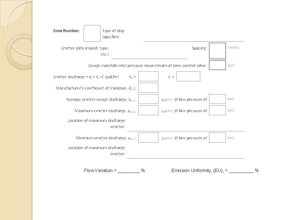
Standard requires Pipe sizes for mains, submains, and laterals shall maintain subunit (zone) emission uniformity (EU) within recommended limits Systems shall be designed to provide discharge to any applicator in an irrigation subunit or zone operated simultaneously such that they will not exceed a total variation of 20 percent of the design discharge rate.
 emission uniformity (EU) within recommended limits Systems shall be designed to provide discharge to any applicator in an irrigation subunit or zone operated simultaneously such that they will not exceed a total variation of 20 percent of the design discharge rate.")
20
Design objective Limit the pressure differential to maintain the desired EU and flow variation What effects the pressure differential ◦ Lateral length and diameter ◦ Manifold location ◦ slope

21
Four Cases

22
Allowable pressure loss (subunit) This applies to both the lateral and subunit. Most of the friction loss occurs in the first 40% of the lateral or manifold D P s =allowable pressure loss for subunit P a = average emitter pressure P n = minimum emitter pressure

23
Emission Uniformity

24
Q is related to Pressure

25
Hydraulics Limited lateral losses to 0.5 D P s Equation for estimating ◦ Darcy-Weisbach(best) ◦ Hazen-Williams ◦ Watters-Keller ( easiest, used in NRCS manuals )
 ◦ Hazen-Williams ◦ Watters-Keller ( easiest, used in NRCS manuals )")
26
C factorPipe diameter (in) 130≤ 1 140< 3 150≥ 3 130Lay flat Hazen-Williams equation hf =friction loss (ft) F = multiple outlet factor Q = flow rate (gpm) C = friction coefficient D = inside diameter of the pipe (in) L = pipe length (ft)
 130≤ 1 140< 3 150≥ 3 130Lay flat Hazen-Williams equation hf =friction loss (ft) F = multiple outlet factor Q = flow rate (gpm) C = friction coefficient D = inside diameter of the pipe (in) L = pipe length (ft)")
27
Watters-Keller equation hf = friction loss (ft) K = constant (.00133 for pipe 5”) F = multiple outlet factor L = pipe length (ft) Q = flow rate (gpm) D = inside pipe diameter (in)
 K = constant ( for pipe 5 ) F = multiple outlet factor L = pipe length (ft) Q = flow rate (gpm) D = inside pipe diameter (in)")
28
Multiple outlet factors Number of outlets F F 1.85 1 1.75 2 1.85 1 1.75 2 1234567812345678 1.00 0.64 0.54 0.49 0.46 0.44 0.43 0.42 1.00 0.65 0.55 0.50 0.47 0.45 0.44 0.43 9 10-11 12-15 16-20 21-30 31-70 >70 0.41 0.40 0.39 0.38 0.37 0.36 0.42 0.41 0.40 0.39 0.38 0.37 0.36

29
Adjust length for barb and other minor losses

30
Adjusted length L’ = adjusted lateral length (ft) L = lateral length (ft) Se = emitter spacing (ft) fe = barb loss (ft)
 L = lateral length (ft) Se = emitter spacing (ft) fe = barb loss (ft)")
31
Start with average lateral

32
Pressure Tanks

33
Practice problem

Similar presentations