Download presentation
Presentation is loading. Please wait.

1
R. Sharma*, A. Langley ** M. Herrera*, J. Geehan*
Indian Ocean Bigeye Tuna Stock Assessment: Weighting length composition versus CPUE data; Issues on Longline and Purse Seine selectivity R. Sharma*, A. Langley ** M. Herrera*, J. Geehan* * IOTC Secretariat ** IOTC Consultant

2
Overview Data and trends Stock Assessment Approach Used
Sensitivity on: Aggregated fleets versus segregated fleets Data weighting (Eff Sample Size issue) LL selectivity by blocks PS and LL selectivity by blocks Implications on assessment Size composition issue- How do we resolve this
 LL selectivity by blocks. PS and LL selectivity by blocks. Implications on assessment. Size composition issue- How do we resolve this.")
3
Bigeye tuna: Catch (i)
")
4
Bigeye tuna: Catch (ii)
1970’s 1990’s 2000’s 2010 2011

5
Bigeye tuna: Catch (iii)
2002/06 - Q1 2002/06 – Q2 2002/06 – Q3 2002/06 – Q4 Q1 2011 – Q2 2011 – Q3 2011 – Q4

6
Bigeye tuna: Average weight
Purse seine Associated school Free-school All fisheries Small (<15kg) Medium (15-30 kg) Large (>30 kg) Small (<15 kg) Longline Japan Longline Taiwan,China
 Medium (15-30 kg) Large (>30 kg) Small (<15 kg) Longline Japan. Longline Taiwan,China.")
7
Bigeye tuna: Tagging data
35,997 BET released to 5,740 recovered (representing ≈16% of the releases), the majority by PS in area 1.
, the majority by PS in area 1.")
9
Bigeye tuna: Data Summary
Total catches have been around 80,000 t in recent years, well below previous years catches Marked drop in catches in main BET fishing grounds (Area 1) Almost no longline BET catch in area 1 in (Piracy) Increased contribution of coastal fleets to catches of bigeye tuna following the development of new fisheries using handlines, coastal longlines, and trolling (some around anchored FADs) Higher contribution of surface fisheries to total catches Drop in average weight
 Almost no longline BET catch in area 1 in (Piracy) Increased contribution of coastal fleets to catches of bigeye tuna following the development of new fisheries using handlines, coastal longlines, and trolling (some around anchored FADs) Higher contribution of surface fisheries to total catches Drop in average weight.")
10
The Assessment Approach Used
SS-III 3 area and One Area Assessment Focus on final model used (One Area Assessment). Base model used LL (Area 1) Logistic Base model used LL (Area 2 and 3) Double Normal. Base model used PSLS (Double Normal). CPUE and Length composition weighting issues.
. Base model used LL (Area 1) Logistic. Base model used LL (Area 2 and 3) Double Normal. Base model used PSLS (Double Normal). CPUE and Length composition weighting issues.")
13
Comparing the Aggregated model versus the segregated model-I
Year Quarter 101 = (Q1) Aggregated Fisheries Segregated Fisheries
 Aggregated Fisheries. Segregated Fisheries.")
14
Comparing the Aggregated model versus the segregated model-II
Aggregated Fisheries Segregated Fisheries

15
Diagnostics-III Aggregated Model

16
Segregated Model

18
Changing effective sample sizes-Segregated Model

19
Changing effective sample sizes-Segregated Model

22
Time Varying Selectivity -LL and PSLS Higher Eff SS

25
Marginal improvement in FL2, LL2 and PSLS1

30
Overall effects on assessment

36
SBMSY Max C ~ 140,000 T in 2002

37
How do we resolve these discrepancies
For now we are using the simple model without weighting length comp data. Investigating issues on sampling and reporting data.

38
Length (2 cm size classes)
Taiwan, China – Big Eye size frequencies distribution (percentiles within each year) Low % High % Length (2 cm size classes) Taiwan, China
 Low % High % Length (2 cm size classes) Taiwan, China.")
39
Size frequency data, 5 x 5 grid
Taiwan, China BE: spatial pattern of SF data Analysis of the spatial pattern pre-2002 are limited by small sample sizes for these years. No overriding pattern can easily be seen. Post-2002 show greater consistency in average weights in each area, with the highest values concentrated in the Arabian Sea area and north-west Indian Ocean. Size frequency data, 5 x 5 grid

40
Bigeye – size-frequency distribution 1980-2011
Between 2001 until 2009 there is noticeable increase in the kurtosis values, caused by the relative narrowing range of size classes recorded by the samples. The overall average weight for these years generally increases – peaking at around 55kg – as the percentage fish recorded in smaller length classes decreases, and the proportion of mid to larger fish increases.

41
Taiwan, China: Bigeye

43
Taiwan, China & Japan: Bigeye

44
Bigeye Size-frequency (SF) data: key points
A number of issues were identified with SF data for Bigeye, including: low sample numbers for catch at size until around 2002; for years where sampling numbers improve ( ) a narrowing of the size-frequency distribution, with a general shift towards samples containing higher proportions of mid to large sized fish (see distribution heatmap on previous slide); as a consequence of the shift in distribution, a relatively large increase in average weight from around 35kg in 2000 to over 55kg by 2006. Size data collected after 2001 appear to have a systematically different size profile to data before 2001, and which needs to be explored more to understand the cause of the sharp rise in the trend of average weight. One suggestion may be the effect of the introduction of quota (weight) limits, i.e., that only fish above a certain size suitable for export market are measured (compared to Catch and Effort which records all sizes); alternatively, issues with the conversion factors from gilled and gutted to live weight; or changes to the reporting system introduced around this time.
 a narrowing of the size-frequency distribution, with a general shift towards samples containing higher proportions of mid to large sized fish (see distribution heatmap on previous slide); as a consequence of the shift in distribution, a relatively large increase in average weight from around 35kg in 2000 to over 55kg by Size data collected after 2001 appear to have a systematically different size profile to data before 2001, and which needs to be explored more to understand the cause of the sharp rise in the trend of average weight. One suggestion may be the effect of the introduction of quota (weight) limits, i.e., that only fish above a certain size suitable for export market are measured (compared to Catch and Effort which records all sizes); alternatively, issues with the conversion factors from gilled and gutted to live weight; or changes to the reporting system introduced around this time.")
45
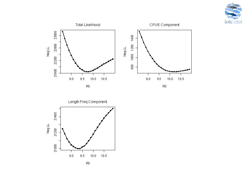
Possible issues in the data sets
Either the Length frequency data is biased & CPUE data is unbiased. CPUE data is biased and LF unbiased. Both CPUE and LF are biased. More thorough examination of these datasets required for the assessment.

46
Overall conclusions Selectivity not as important as the Effective SS estimated on length frequency of catches by fleets. Selectivity is important as the shape used will effect the key reference points estimated. More thorough Need: Resolve average size discrepancies between periods in the LL fisheries as these drive the assessment if weighed high. Interactions with growth and natural mortality poorly understood, and more work needs to be conducted.

47
Acknowledgements Rick Methot for developing the 2 stanza growth curve which we used in the assessment. Ian Taylor for answering obscure questions about SS. Adam Langley for constant advice on assessments. IOTC countries for sharing their data with us. Mark for letting me know about the meeting. ISSF for funding travel.

Similar presentations


 Center for the Advancement of Population.>")


 von Bertalanffy growth parameters using conditional-age-at-length data.>")


 IN THE EASTERN PACIFIC OCEAN January 1975 – December 2006.>")


. Adam Langley, Miguel Herrera and Julien Million.>")