1. Dynamical Systems and Computational Mechanisms Belgium Workshop July 1-2, 2002 Roger Brockett Engineering and Applied Sciences Harvard University

2. Issues and Approach 1. Developments in fields outside electrical engineering and computer science have raised questions about the possibility of carrying out computation in ways other than those based on digital logic. Quantum computing and neuro-computing are examples. 2. When formulated mathematically, these new fields relate to dynamical systems and raise questions in signal processing whose resolution seems to require new methods. 3. Up until now, the statement that computers are dynamical systems of the input/output type has not gotten computer scientists especially excited because it has not yet been shown to have practical consequence or theoretical power. 4. It is my goal here to try to show that this point of view has both explanatory value and is mathematical interest.

3. Outline of the Day 9:30-10-45 Part 1. Examples and Mathematical Background 10:45 - 11:15 Coffee break 11:15 - 12:30 Part 2. Principal components, Neural Nets, and Automata 12:30 - 14:30 Lunch 14:30 - 15:45 Part 3. Precise and Approximate Representation of Numbers 15:45 - 16:15 Coffee break 16:15 - 17:30 Part 4. Quantum Computation

4. Architectural Suggestions from Neuroscience

5. Features of the Counter Flow Cartoon The organization goes from topographic, “high resolution” data, to abstract, and presumably “tree structured” representations in which any continuity would be relative to some “degree of association” topology. The role of long term memory becomes more important as the representation becomes more abstract On the action side, time plays a pivotal role, because of need for animals to react in a timely way. Reflexes are very fast but inflexible. Other actions such as playing football or Bach requires interaction with memory coordination of muscle groups, etc.

6. Some of the Important Sub Systems 1. Filters as streaming processors 2. Topographic (k-dimensional) processing vs. associative processing 3. Analog-to-Digital Conversion, Quantization 4. Label, Categorize, Classify, Cluster, Tokenize. Make a distinction between the problems in which the categories are fixed in advance (non adaptive) and the case where the categories are to be determined on the basis of the data (adaptive). Also distinguish between “flat” and “hierarchical” categorization. In the latter case a tree structure is implicit and in the adaptive case this tree structure must be generated from the data.

7. The Purpose of Labeling is to Simplify Key aspects: Communication, Computation, Reasoning and Storage/Retrieval The simplification invariably means that digitization is a many-to-one mapping. Typically the ambiguity introduced by this mapping is more pronounced at some points of the domain than at others. The ordinary uniformly spaced quantizer q(x) is very precise at the jump points and maximally imprecise elsewhere. We want to put the imprecision where it won’t hurt us. Other widely used maps from a continuum to a discrete set include the mapping from the space of smooth closed curves in a topological space to an element of the fundamental group of that space. This simplification is basic to the use of algebraic topology. It is a many-to-one mapping but it distributes the ambiguity in a rather different way.

8. Example 1: Analog Sorter in Differential Equation Form

9. The Analog Sorter

11. Difficulties with the Cartesian-Lagrangian Point of View The representation of a number by choosing a scale and associating a numerical value with the instantaneous value of a physical quantity such as voltage, current, mole fraction, etc. seems to lack the required robustness in many situations, Examples of alternative representations used in engineering, nature, and mathematics include: 1. The use of elapsed time to represent the number. (How much time does it take for a capacitor to charge up to one volt in a given situation.) 2. How many fixed shape pulses occur in a given period of time. (pulse frequency modulation) 3. Identify a point in a manifold with the maximal ideal it generates in the ring of continuous functions mapping the manifold into some field of numbers. (The algebraic geometry point of view.)

12. Example 2: Topological Representations of Finite Sets Digital electronics represents binary numbers using voltages that are Well separated from each other, whose nominal values are, say, 0 and 3.2 but whose actual values may differ from these if the difference is not too much. Voltages that are in between these values are not allowed, which is to say they correspond to broken systems. Of course transients are allowed but these must be rapid and represent decisive transitions between levels..

13. Classifying Quantizers

14. The Pulse Annulus and its Winding Number The annular characterization allows arbitrary spacing between pulses, a characterization of a set of functions that is very different from, say, the characterization of band-limited functions.

15. Computing with Pulse Representations

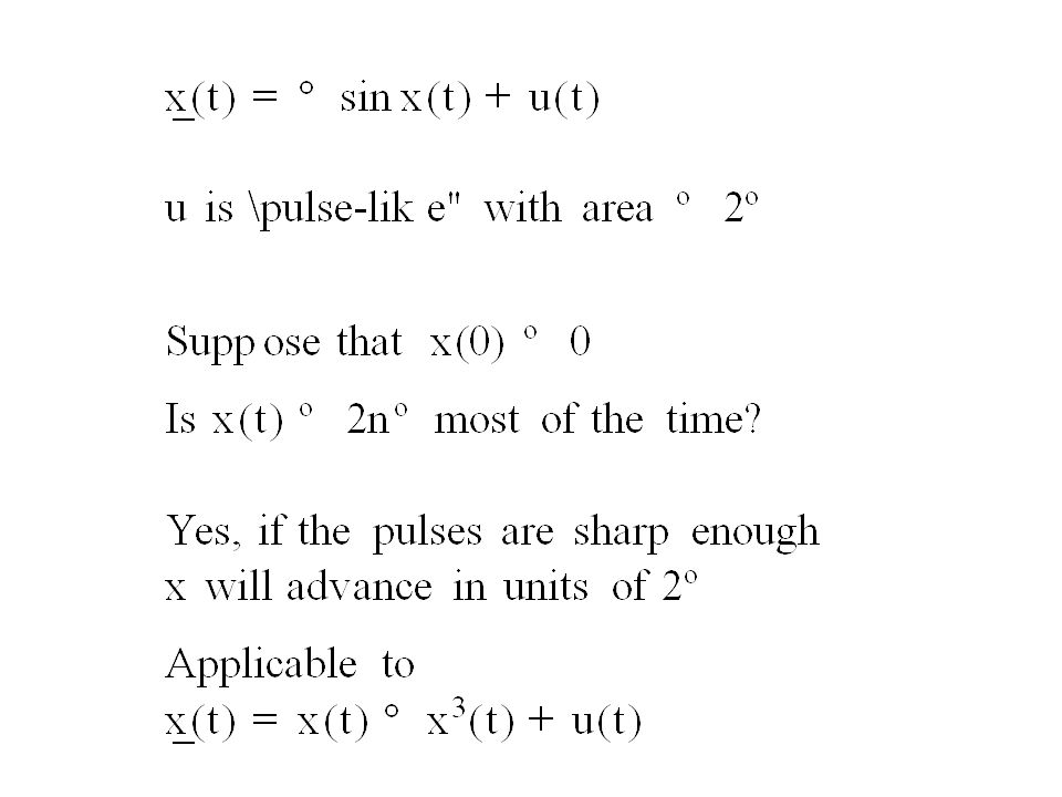
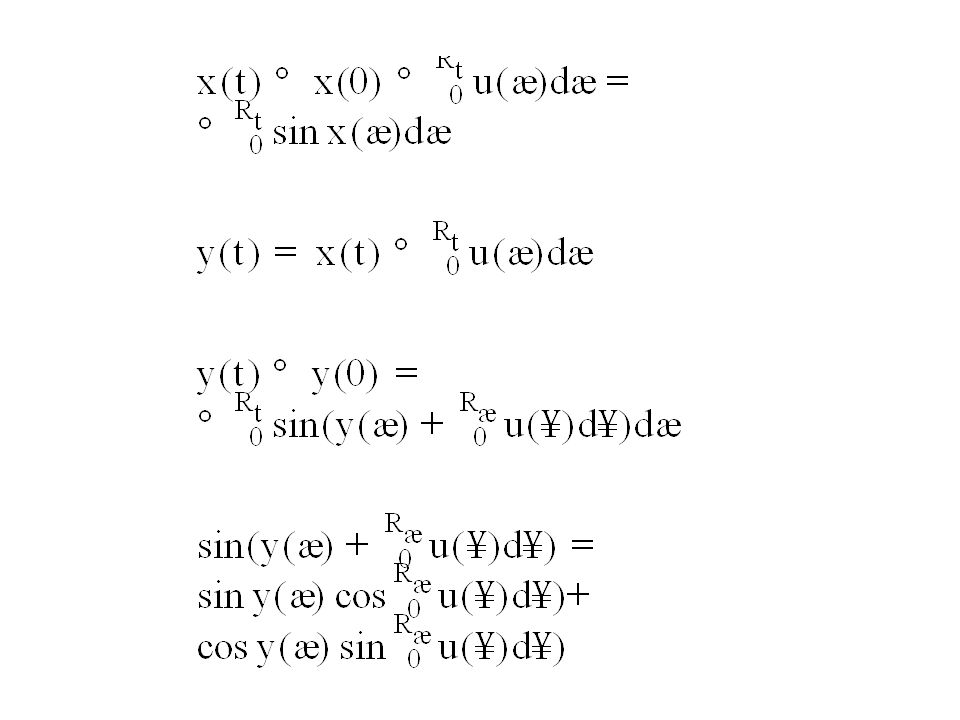
19. Example 3: The Place of Cell Representation An important idea from neuroscience: Representation of numbers via overlapping place cells. Tuning curves determine the rate as a function of the distance to the central point of the particular tuning curve, g i ( ). The vector x is a vector of pulse streams of variable frequency. The frequency of the i th stream is determined by the value of g i (x). Compare with the maximal ideal point of view: The derivative defines An ideal in the ring of real valued continuous functions on the space.

20. Conditional Density as the Be-All and End-All In reasoning about an uncertain world, data is collected and the probability of various underlying causes is then evaluated and compared with the relevant priors. This process is played out in time. When expressed in mathematical form this takes form dp/dt = (A-(1/2)D 2 )p +y(t)Dp or Ap-(1/2)(D-Iy) 2 p With y being the observations and p/(p 1 +p 2 +…p n ) being the conditional probability. The point to be made here is that there is an evolution equation for the conditional probability (or probability density) and that the maximum likelihood estimate is the argmax of p..

21. Conditional Density Flow Takes away More or Less

22. Conditional Density Equation: x Real Valued

23. The Conditional Density Provides a Robust Representation Taken literally, the evolution of the conditional density is an expensive representation of a real number via argmax but it is robust and, in a decision theoretic setting, normally a minimal representation. If we use a suitable approximation it can be thought of as yielding a “digital” representation via histograms, splines or Bezier curves.

24. Place Cells Representation vs. Conditional Density The evolution of the conditional density is not too different from the evolution of the place cell representation if we think of the latter as being some kind of spline representation of the conditional density.

25. Fact: The conditional density for the usual gauss markov process observed with additive white noise evolves as a Gaussian. The argmax of a Gaussian can be computed via the mean. Thus it is possible to convert ordinary differential algorithms into density evolution equations which will do the same calculations. It seems likely that the brute force way of doing this is not the most efficient and from our knowledge of completely integrable systems it seems likely that one can find soliton equations that will perform these calculations robustly. I know of very few results of this kind. Computation with an Argmax (Place Cell) Representation

26. A Distributed (Argmax) Model for Analog Computation

27. The Argmax Representation

28. Example 4: Adjoint Orbits and Mixed Computation The Toda lattice is a restriction of the general isospectral gradient flow dH/dt = [H,[H,N]] (whose natural domain of definition is any adjoint orbit) to the space of tridiagonal symmetric matrices. This flow finds eigenvalues and eigenvectors, (and therefore principal components), sorts, and, via tensoring, can be used as a building block for more specialized computations. Variations include dH/dt = [H,[H,diag(H)]] which flows to a diagonal determined by the initial conditions.

29. Summary of Part 1 1. The distinction between analog signal processing is not as clear- cut as the words might suggest. 2. There are various ways to achieve robustness and the choice of a representation must be adapted to the computational “hardware” available. 3. Cartesian/Lagrangian, homotopy, and place cell (argmax) representations are all used as representation schemes. 4. Examples show that one can compute with any of these representational schemes, but that the first seems to lack the robustness necessary to form a satisfactory basis for a all encompassing theory and needs to be supplemented.