1. Semiconductor Devices III Physics 355

2. Transistors in CPUs Moore’s Law (1965): the number of components in an integrated circuit will double every year; and in its present form that time constant is usually quoted as 18 months although, at least for Intel's CPUs, the number of transistors in a CPU doubles roughly every two years

3. Field Effect Transistors The npn and pnp junction type transistors lead the way to modern electronic devices, but there are disadvantages to their use. For example, the signal is input to the low impedance base and the base-emitter diode is forward biased. Another device achieved transistor action with the input diode junction reversed biased, and this device is called a "field effect transistor" or a "junction field effect transistor", JFET. With the reverse biased input junction, it has a very high input impedance. A high input impedance minimizes the interference with or "loading" of the signal source when a measurement is made.

4. JFETs: Operation JFETs require a drain source voltage, +V DD and a gate-source bias voltage, V GS The drain supply voltage causes a current I D (the drain current) to flow through the n channel. The drain current is made up of the majority carriers, in this case, electrons. The value of the drain current is dependent on both +V DD and V GS. An input of zero volts, reverse biases the p-n junction, resulting in a maximum channel width and maximum source to drain current.

5. JFETs

6. JFETs: Common Source C1C1 R1R1 Source R2R2 C2C2 Input C3C3 R3R3 +V DD Output Most common configuration is shown. The source is grounded and common to both the input and output signals.

7. MOSFETs The n-type Metal-Oxide- Semiconductor Field-Effect- Transistor (MOSFET) consists of a source and a drain, two highly conducting n-type semiconductor regions which are isolated from the p-type substrate by reversed- biased p-n diodes. A metal (or poly-crystalline) gate covers the region between source and drain, but is separated from the semiconductor by the gate oxide. These have very high impedances - in the range 10 9 to 10 14 ohms.

8. MOSFETs

9. MOSFETs: Models Linear The linear model describes the behavior of a MOSFET biased with a small drain-to-source voltage. As the name suggests, the MOSFET, acts as a linear device, more specifically a linear resistor whose resistance can be modulated by changing the gate-to-source voltage. In this regime the MOSFET can be used as a switch for analog signals or as an analog multiplier. Quadratic The quadratic model includes the gradual change of the charge in the inversion layer between the source and the drain due to the fact that the channel voltage varies from the source voltage to the drain voltage. Variable Depletion Layer The variable depletion layer model includes, in addition to the gradual change of the inversion layer charge, the variation of the charge in the depletion layer between the inversion layer and the substrate. This model is required to understand the body or substrate bias effect.

10. MOSFETs: Linear Model The general expression for the drain current equals the total charge in the inversion layer divided by the time the carriers need to flow from the source to the drain: where Q inv is the inversion layer charge per unit area, W is the gate width, L is the gate length and t r is the transit time. If the velocity of the carriers is constant between source and drain, the transit time equals: where the velocity equals the product of the mobility and the electric field:

11. The constant velocity also implies a constant electric field so that the field equals the drain-source voltage divided by the gate length. This leads to the following expression for the drain current: MOSFETs: Linear Model We now make an assumption about the inversion layer charge density, namely that it is constant between source and drain and that the charge density in the inversion layer is given by the product of the capacitance per unit area and the gate-to-source voltage minus the threshold voltage: The charge is zero if the gate voltage is lower than the threshold voltage. Replacing the inversion layer charge density in the expression for the drain current yields the linear model:

12. MOSFETs: Linear Model

13. MOSFETs: Quadratic Model Considering a small section within the device with width dx and channel voltage V C + V S one can still use the linear model, yielding: where the drain-source voltage is replaced by the change in channel voltage over a distance dx, namely dV C. Both sides of the equation can be integrated from the source to the drain, so that x varies from 0 to the gate length, L, and the channel voltage V C varies from 0 to the drain-source voltage, V DS. Using the fact that the DC drain current is constant throughout the device one obtains the following expression:

14. MOSFETs: Quadratic Model Drain current saturation therefore occurs when the drain-to-source voltage equals the gate-to-source voltage minus the threshold voltage. The value of the drain current is then given by the following equation: The quadratic model explains the typical current-voltage characteristics of a MOSFET which are normally plotted for different gate-to-source voltages. An example is shown in the figure above. The saturation occurs to the right of the dotted line which is given by I D =  C ox W/L V DS 2. The dotted line separates the quadratic region of operation on the left from the saturation region on the right.

15. MOSFETs: Variable Depletion Model The figure shows a clear difference between the two models: the quadratic model yields a larger drain current compared to the more accurate variable depletion layer charge model. However, because of its simplicity, the quadratic model is widely used. Fitting parameters are often used instead of the actual device parameters in order to more closely describe the measured characteristics.

16. Solid State Lasers

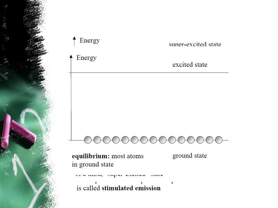
17. Non-Lasers

19. Lasers

20. Solid State Lasers Ruby

21. Solid State Lasers: Nd:YAG Neodymium-Doped : Yttrium Aluminium Garnet

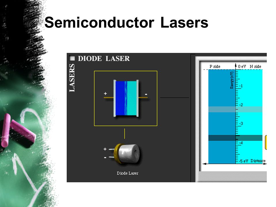
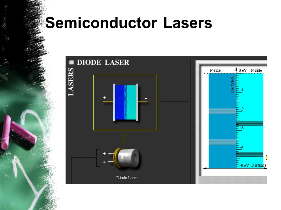
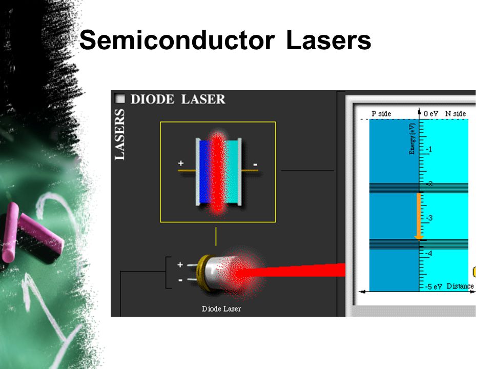
22. Semiconductor Lasers