CE 579: STRUCTRAL STABILITY AND DESIGN

CE 579: STRUCTRAL STABILITY AND DESIGN
Amit H. Varma Assistant Professor School of Civil Engineering Purdue University Ph. No. (765) Office hours: M-W-F 9:00-11:30 a.m.

Chapter 1. Introduction to Structural Stability
OUTLINE Definition of stability Types of instability Methods of stability analyses Examples – small deflection analyses Examples – large deflection analyses Examples – imperfect systems Design of steel structures

STABILITY DEFINITION Change in geometry of a structure or structural component under compression – resulting in loss of ability to resist loading is defined as instability in the book. Instability can lead to catastrophic failure  must be accounted in design. Instability is a strength-related limit state. Why did we define instability instead of stability? Seem strange! Stability is not easy to define. Every structure is in equilibrium – static or dynamic. If it is not in equilibrium, the body will be in motion or a mechanism. A mechanism cannot resist loads and is of no use to the civil engineer. Stability qualifies the state of equilibrium of a structure. Whether it is in stable or unstable equilibrium.

STABILITY DEFINITION Structure is in stable equilibrium when small perturbations do not cause large movements like a mechanism. Structure vibrates about it equilibrium position. Structure is in unstable equilibrium when small perturbations produce large movements – and the structure never returns to its original equilibrium position. Structure is in neutral equilibrium when we cant decide whether it is in stable or unstable equilibrium. Small perturbation cause large movements – but the structure can be brought back to its original equilibrium position with no work. Thus, stability talks about the equilibrium state of the structure. The definition of stability had nothing to do with a change in the geometry of the structure under compression – seems strange!

STABILITY DEFINITION

BUCKLING Vs. STABILITY Change in geometry of structure under compression – that results in its ability to resist loads – called instability. Not true – this is called buckling. Buckling is a phenomenon that can occur for structures under compressive loads. The structure deforms and is in stable equilibrium in state-1. As the load increases, the structure suddenly changes to deformation state-2 at some critical load Pcr. The structure buckles from state-1 to state-2, where state-2 is orthogonal (has nothing to do, or independent) with state-1. What has buckling to do with stability? The question is - Is the equilibrium in state-2 stable or unstable? Usually, state-2 after buckling is either neutral or unstable equilibrium

BUCKLING P=Pcr P<Pcr P>Pcr P d P P P d

BUCKLING Vs. STABILITY Thus, there are two topics we will be interested in this course Buckling – Sudden change in deformation from state-1 to state-2 Stability of equilibrium – As the loads acting on the structure are increased, when does the equilibrium state become unstable? The equilibrium state becomes unstable due to: Large deformations of the structure Inelasticity of the structural materials We will look at both of these topics for Columns Beams Beam-Columns Structural Frames

TYPES OF INSTABILITY Structure subjected to compressive forces can undergo: Buckling – bifurcation of equilibrium from deformation state-1 to state-2. Bifurcation buckling occurs for columns, beams, and symmetric frames under gravity loads only Failure due to instability of equilibrium state-1 due to large deformations or material inelasticity Elastic instability occurs for beam-columns, and frames subjected to gravity and lateral loads. Inelastic instability can occur for all members and the frame. We will study all of this in this course because we don’t want our designed structure to buckle or fail by instability – both of which are strength limit states.

TYPES OF INSTABILITY BIFURCATION BUCKLING
Member or structure subjected to loads. As the load is increased, it reaches a critical value where: The deformation changes suddenly from state-1 to state-2. And, the equilibrium load-deformation path bifurcates. Critical buckling load when the load-deformation path bifurcates Primary load-deformation path before buckling Secondary load-deformation path post buckling Is the post-buckling path stable or unstable?

SYMMETRIC BIFURCATION
Post-buckling load-deform. paths are symmetric about load axis. If the load capacity increases after buckling then stable symmetric bifurcation. If the load capacity decreases after buckling then unstable symmetric bifurcation.

ASYMMETRIC BIFURCATION
Post-buckling behavior that is asymmetric about load axis.

INSTABILITY FAILURE There is no bifurcation of the load-deformation path. The deformation stays in state-1 throughout The structure stiffness decreases as the loads are increased. The change is stiffness is due to large deformations and / or material inelasticity. The structure stiffness decreases to zero and becomes negative. The load capacity is reached when the stiffness becomes zero. Neutral equilibrium when stiffness becomes zero and unstable equilibrium when stiffness is negative. Structural stability failure – when stiffness becomes negative.

Instability due to material and geometric nonlinearity
INSTABILITY FAILURE FAILURE OF BEAM-COLUMNS P M K=0 M K<0 d K M d P No bifurcation. Instability due to material and geometric nonlinearity

INSTABILITY FAILURE Snap-through buckling P Snap-through d

INSTABILITY FAILURE Shell Buckling failure – very sensitive to imperfections

OUTLINE Definition of stability Types of instability Methods of stability analyses Examples – small deflection analyses Examples – large deflection analyses Examples – imperfect systems Design of steel structures

METHODS OF STABILITY ANALYSES
Bifurcation approach – consists of writing the equation of equilibrium and solving it to determine the onset of buckling. Energy approach – consists of writing the equation expressing the complete potential energy of the system. Analyzing this total potential energy to establish equilibrium and examine stability of the equilibrium state. Dynamic approach – consists of writing the equation of dynamic equilibrium of the system. Solving the equation to determine the natural frequency (w) of the system. Instability corresponds to the reduction of w to zero.

STABILITY ANALYSES Each method has its advantages and disadvantages. In fact, you can use different methods to answer different questions The bifurcation approach is appropriate for determining the critical buckling load for a (perfect) system subjected to loads. The deformations are usually assumed to be small. The system must not have any imperfections. It cannot provide any information regarding the post-buckling load-deformation path. The energy approach is the best when establishing the equilibrium equation and examining its stability The deformations can be small or large. The system can have imperfections. It provides information regarding the post-buckling path if large deformations are assumed The major limitation is that it requires the assumption of the deformation state, and it should include all possible degrees of freedom.

STABILITY ANALYSIS The dynamic method is very powerful, but we will not use it in this class at all. Remember, it though when you take the course in dynamics or earthquake engineering In this class, you will learn that the loads acting on a structure change its stiffness. This is significant – you have not seen it before. What happens when an axial load is acting on the beam. The stiffness will no longer remain 4EI/L and 2EI/L. Instead, it will decrease. The reduced stiffness will reduce the natural frequency and period elongation. You will see these in your dynamics and earthquake engineering class. qa Ma Mb P

STABILITY ANALYSIS FOR ANY KIND OF BUCKLING OR STABILITY ANALYSIS – NEED TO DRAW THE FREE BODY DIAGRAM OF THE DEFORMED STRUCTURE. WRITE THE EQUATION OF STATIC EQUILIBRIUM IN THE DEFORMED STATE WRITE THE ENERGY EQUATION IN THE DEFORMED STATE TOO. THIS IS CENTRAL TO THE TOPIC OF STABILITY ANALYSIS NO STABILITY ANALYSIS CAN BE PERFORMED IF THE FREE BODY DIAGRAM IS IN THE UNDEFORMED STATE

BIFURCATION ANALYSIS Always a small deflection analysis
To determine Pcr buckling load Need to assume buckled shape (state 2) to calculate Example 1 – Rigid bar supported by rotational spring Step 1 - Assume a deformed shape that activates all possible d.o.f. P k L Rigid bar subjected to axial force P Rotationally restrained at end q L P L cosq kq L (1-cosq)

BIFURCATION ANALYSIS L P Write the equation of static equilibrium in the deformed state Thus, the structure will be in static equilibrium in the deformed state when P = Pcr = k/L When P<Pcr, the structure will not be in the deformed state. The structure will buckle into the deformed state when P=Pcr kq L sinq q L cosq L (1-cosq)

BIFURCATION ANALYSIS Example 2 - Rigid bar supported by translational spring at end P k L Assume deformed state that activates all possible d.o.f. Draw FBD in the deformed state P L q L (1-cosq) L cosq k L sinq L sinq O

BIFURCATION ANALYSIS Write equations of static equilibrium in deformed state P L L sinq q O k L sinq L cosq L (1-cosq) Thus, the structure will be in static equilibrium in the deformed state when P = Pcr = k L. When P<Pcr, the structure will not be in the deformed state. The structure will buckle into the deformed state when P=Pcr

BIFURCATION ANALYSIS Example 3 – Three rigid bar system with two rotational springs P P k k A D B C L L L Assume deformed state that activates all possible d.o.f. Draw FBD in the deformed state P A D k L q1 q2 L sin q1 L sin q2 B C (q1 – q2) Assume small deformations. Therefore, sinq=q

BIFURCATION ANALYSIS Write equations of static equilibrium in deformed state P k P k q2 A q1 L sin q2 D L sin q1 (q1 – q2) L L C B (q1 – q2) k P P q2 L sin q2 D q2-(q1 – q2) L A q1 C L sin q1 L k(2q2-q1) k(2q1-q2) q1+(q1-q2) B

BIFURCATION ANALYSIS Equations of Static Equilibrium
Therefore either q1 and q2 are equal to zero or the determinant of the coefficient matrix is equal to zero. When q1 and q2 are not equal to zero – that is when buckling occurs – the coefficient matrix determinant has to be equal to zero for equil. Take a look at the matrix equation. It is of the form [A] {x}={0}. It can also be rewritten as ([K]-l[I]){x}={0}

BIFURCATION ANALYSIS This is the classical eigenvalue problem. ([K]-l[I]){x}={0}. We are searching for the eigenvalues (l) of the stiffness matrix [K]. These eigenvalues cause the stiffness matrix to become singular Singular stiffness matrix means that it has a zero value, which means that the determinant of the matrix is equal to zero. Smallest value of Pcr will govern. Therefore, Pcr=k/L

BIFURCATION ANALYSIS Each eigenvalue or critical buckling load (Pcr) corresponds to a buckling shape that can be determined as follows Pcr=k/L. Therefore substitute in the equations to determine q1 and q2 All we could find is the relationship between q1 and q2. Not their specific values. Remember that this is a small deflection analysis. So, the values are negligible. What we have found is the buckling shape – not its magnitude. The buckling mode is such that q1=q2  Symmetric buckling mode P k k P A q1 q2=q1 D L L B C

BIFURCATION ANALYSIS Second eigenvalue was Pcr=3k/L. Therefore substitute in the equations to determine q1 and q2 All we could find is the relationship between q1 and q2. Not their specific values. Remember that this is a small deflection analysis. So, the values are negligible. What we have found is the buckling shape – not its magnitude. The buckling mode is such that q1=-q2  Antisymmetric buckling mode C L P k k q2=-q1 P A q1 D L B

BIFURCATION ANALYSIS Homework No. 1 Problem 1.1 Problem 1.3
All problems from the textbook on Stability by W.F. Chen

OUTLINE Definition of stability Types of instability Methods of stability analyses Bifurcation analysis examples – small deflection analyses Energy method Examples – small deflection analyses Examples – large deflection analyses Examples – imperfect systems Design of steel structures

ENERGY METHOD We will currently look at the use of the energy method for an elastic system subjected to conservative forces. Total potential energy of the system – P – depends on the work done by the external forces (We) and the strain energy stored in the system (U). P = U - We. For the system to be in equilibrium, its total potential energy P must be stationary. That is, the first derivative of P must be equal to zero. Investigate higher order derivatives of the total potential energy to examine the stability of the equilibrium state, i.e., whether the equilibrium is stable or unstable

ENERGY METHD The energy method is the best for establishing the equilibrium equation and examining its stability The deformations can be small or large. The system can have imperfections. It provides information regarding the post-buckling path if large deformations are assumed The major limitation is that it requires the assumption of the deformation state, and it should include all possible degrees of freedom.

ENERGY METHOD Example 1 – Rigid bar supported by rotational spring
Assume small deflection theory Step 1 - Assume a deformed shape that activates all possible d.o.f. P k L Rigid bar subjected to axial force P Rotationally restrained at end q L P L cosq kq L (1-cosq)

ENERGY METHOD – SMALL DEFLECTIONS
L (1-cosq) q L P L cosq kq L sinq Write the equation representing the total potential energy of system

The energy method predicts that buckling will occur at the same load Pcr as the bifurcation analysis method. At Pcr, the system will be in equilibrium in the deformed. Examine the stability by considering further derivatives of the total potential energy This is a small deflection analysis. Hence q will be  zero. In this type of analysis, the further derivatives of P examine the stability of the initial state-1 (when q =0)

In state-1, stable when P<Pcr, unstable when P>Pcr No idea about state during buckling. No idea about post-buckling equilibrium path or its stability. Pcr q P Stable Unstable Indeterminate

ENERGY METHOD – LARGE DEFLECTIONS
Example 1 – Large deflection analysis (rigid bar with rotational spring) L (1-cosq) q L P L cosq kq L sinq

Large deflection analysis See the post-buckling load-displacement path shown below The load carrying capacity increases after buckling at Pcr Pcr is where q  0

Large deflection analysis – Examine the stability of equilibrium using higher order derivatives of P

At q =0, the second derivative of P=0. Therefore, inconclusive. Consider the Taylor series expansion of P at q=0 Determine the first non-zero term of P, Since the first non-zero term is > 0, the state is stable at P=Pcr and q=0

STABLE STABLE STABLE

ENERGY METHOD – IMPERFECT SYSTEMS
Consider example 1 – but as a system with imperfections The initial imperfection given by the angle q0 as shown below The free body diagram of the deformed system is shown below P k q0 L L cos(q0) L (cosq0-cosq) L P L cosq k(q-q0) L sinq q q0

L (cosq0-cosq) L P L cosq k(q-q0) L sinq q q0

ENERGY METHODS – IMPERFECT SYSTEMS
As shown in the figure, deflection starts as soon as loads are applied. There is no bifurcation of load-deformation path for imperfect systems. The load-deformation path remains in the same state through-out. The smaller the imperfection magnitude, the close the load-deformation paths to the perfect system load –deformation path The magnitude of load, is influenced significantly by the imperfection magnitude. All real systems have imperfections. They may be very small but will be there The magnitude of imperfection is not easy to know or guess. Hence if a perfect system analysis is done, the results will be close for an imperfect system with small imperfections

Examine the stability of the imperfect system using higher order derivatives of P Which is always true, hence always in STABLE EQUILIBRIUM

Example 2 - Rigid bar supported by translational spring at end P k L Assume deformed state that activates all possible d.o.f. Draw FBD in the deformed state P L q L (1-cosq) L cosq k L sinq L sinq O

Write the equation representing the total potential energy of system P L q L (1-cosq) L cosq L sinq k L sinq O

The energy method predicts that buckling will occur at the same load Pcr as the bifurcation analysis method. At Pcr, the system will be in equilibrium in the deformed. Examine the stability by considering further derivatives of the total potential energy This is a small deflection analysis. Hence q will be  zero. In this type of analysis, the further derivatives of P examine the stability of the initial state-1 (when q =0)

Write the equation representing the total potential energy of system P L L sinq q O L cosq L (1-cosq)

Large deflection analysis See the post-buckling load-displacement path shown below The load carrying capacity decreases after buckling at Pcr Pcr is where q  0

Large deflection analysis – Examine the stability of equilibrium using higher order derivatives of P

At q =0, the second derivative of P=0. Therefore, inconclusive. Consider the Taylor series expansion of P at q=0 Determine the first non-zero term of P, Since the first non-zero term is < 0, the state is unstable at P=Pcr and q=0

UNSTABLE UNSTABLE UNSTABLE

ENERGY METHOD - IMPERFECTIONS
Consider example 2 – but as a system with imperfections The initial imperfection given by the angle q0 as shown below The free body diagram of the deformed system is shown below P q0 L k L cos(q0) P L q L (cosq0-cosq) L cosq L sinq O q0 L sinq0

L q L (cosq0-cosq) L cosq L sinq O q0 L sinq0

Envelope of peak loads Pmax

As shown in the figure, deflection starts as soon as loads are applied. There is no bifurcation of load-deformation path for imperfect systems. The load-deformation path remains in the same state through-out. The smaller the imperfection magnitude, the close the load-deformation paths to the perfect system load –deformation path. The magnitude of load, is influenced significantly by the imperfection magnitude. All real systems have imperfections. They may be very small but will be there The magnitude of imperfection is not easy to know or guess. Hence if a perfect system analysis is done, the results will be close for an imperfect system with small imperfections. However, for an unstable system – the effects of imperfections may be too large.

Examine the stability of the imperfect system using higher order derivatives of P

Chapter 2. – Second-Order Differential Equations
This chapter focuses on deriving second-order differential equations governing the behavior of elastic members 2.1 – First order differential equations 2.2 – Second-order differential equations

2.1 First-Order Differential Equations
Governing the behavior of structural members Elastic, Homogenous, and Isotropic Strains and deformations are really small – small deflection theory Equations of equilibrium in undeformed state Consider the behavior of a beam subjected to bending and axial forces

Assume tensile forces are positive and moments are positive according to the right-hand rule Longitudinal stress due to bending This is true when the x-y axis system is a centroidal and principal axis system.

The corresponding strain is If P=My=0, then Plane-sections remain plane and perpendicular to centroidal axis before and after bending The measure of bending is curvature f which denotes the change in the slope of the centroidal axis between two point dz apart

Shear Stresses due to bending

Differential equations of bending Assume principle of superposition Treat forces and deformations in y-z and x-z plane seperately Both the end shears and qy act in a plane parallel to the y-z plane through the shear center S

Differential equations of bending Fourth-order differential equations using first-order force-deformation theory

Torsion behavior – Pure and Warping Torsion
Torsion behavior – uncoupled from bending behavior Thin walled open cross-section subjected to torsional moment This moment will cause twisting and warping of the cross-section. The cross-section will undergo pure and warping torsion behavior. Pure torsion will produce only shear stresses in the section Warping torsion will produce both longitudinal and shear stresses The internal moment produced by the pure torsion response will be equal to Msv and the internal moment produced by the warping torsion response will be equal to Mw. The external moment will be equilibriated by the produced internal moments MZ=MSV + MW

Pure and Warping Torsion
MZ=MSV + MW Where, MSV = G KT f′ and MW = - E Iw f"‘ MSV = Pure or Saint Venant’s torsion moment KT = J = Torsional constant = f is the angle of twist of the cross-section. It is a function of z. IW is the warping moment of inertia of the cross-section. This is a new cross-sectional property you may not have seen before. MZ = G KT f′ - E Iw f"‘ ……… (3), differential equation of torsion

Pure Torsion Differential Equation
Lets look closely at pure or Saint Venant’s torsion. This occurs when the warping of the cross-section is unrestrained or absent For a circular cross-section – warping is absent. For thin-walled open cross-sections, warping will occur. The out of plane warping deformation w can be calculated using an equation I will not show.

Pure Torsion Stresses The torsional shear stresses vary linearly about the center of the thin plate tsv

Warping deformations The warping produced by pure torsion can be restrained by the: (a) end conditions, or (b) variation in the applied torsional moment (non-uniform moment) The restraint to out-of-plane warping deformations will produce longitudinal stresses (sw) , and their variation along the length will produce warping shear stresses (tw) .

Warping Torsion Differential Equation
Lets take a look at an approximate derivation of the warping torsion differential equation. This is valid only for I and C shaped sections.

Torsion Differential Equation Solution
Torsion differential equation MZ=MSV+MW = G KT f’- E IW f’’’ This differential equation is for the case of concentrated torque Torsion differential equation for the case of distributed torque The coefficients C C6 can be obtained using end conditions

Torsion Differential Equation Solution
Torsionally fixed end conditions are given by These imply that twisting and warping at the fixed end are fully restrained. Therefore, equal to zero. Torsionally pinned or simply-supported end conditions given by: These imply that at the pinned end twisting is fully restrained (f=0) and warping is unrestrained or free. Therefore, sW=0 f’’=0 Torsionally free end conditions given by f’=f’’ = f’’’= 0 These imply that at the free end, the section is free to warp and there are no warping normal or shear stresses. Results for various torsional loading conditions given in the AISC Design Guide 9 – can be obtained from my private site

Warping Torsion Stresses
Restraint to warping produces longitudinal and shear stresses The variation of these stresses over the section is defined by the section property Wn and Sw The variation of these stresses along the length of the beam is defined by the derivatives of f. Note that a major difference between bending and torsional behavior is The stress variation along length for torsion is defined by derivatives of f, which cannot be obtained using force equilibrium. The stress variation along length for bending is defined by derivatives of v, which can be obtained using force equilibrium (M, V diagrams).

Torsional Stresses

Torsional Section Properties for I and C Shapes

f and derivatives for concentrated torque at midspan

Summary of first order differential equations
NOTES: Three uncoupled differential equations Elastic material – first order force-deformation theory Small deflections only Assumes – no influence of one force on other deformations Equations of equilibrium in the undeformed state.

HOMEWORK # 3 Consider the 22 ft. long simply-supported W18x65 wide flange beam shown in Figure 1 below. It is subjected to a uniformly distributed load of 1k/ft that is placed with an eccentricity of 3 in. with respect to the centroid (and shear center). At the mid-span and the end support cross-sections, calculate the magnitude and distribution of: Normal and shear stresses due to bending Shear stresses due to pure torsion Warping normal and shear stresses over the cross-section. Provide sketches and tables of the individual normal and shear stress distributions for each case. Superimpose the bending and torsional stress-states to determine the magnitude and location of maximum stresses.

HOMEWORK # 2 22 ft. 3in. Span W18x65 Cross-section

Chapter 2. – Second-Order Differential Equations
This chapter focuses on deriving second-order differential equations governing the behavior of elastic members 2.1 – First order differential equations 2.2 – Second-order differential equations

2.2 Second-Order Differential Equations
Governing the behavior of structural members Elastic, Homogenous, and Isotropic Strains and deformations are really small – small deflection theory Equations of equilibrium in deformed state The deformations and internal forces are no longer independent. They must be combined to consider effects. Consider the behavior of a member subjected to combined axial forces and bending moments at the ends. No torsional forces are applied explicitly – because that is very rare for CE structures.

Member model and loading conditions
Member is initially straight and prismatic. It has a thin-walled open cross-section Member ends are pinned and prevented from translation. The forces are applied only at the member ends These consist only of axial and bending moment forces P, MTX, MTY, MBX, MBY Assume elastic behavior with small deflections Right-hand rule for positive moments and reactions and P assumed positive.

Member displacements (cross-sectional)
Consider the middle line of thin-walled cross-section x and y are principal coordinates through centroid C Q is any point on the middle line. It has coordinates (x, y). Shear center S coordinates are (xo, y0) Shear center S displacements are u, v, and f

Member displacements (cross-sectional)
Displacements of Q are: uQ = u + a f sin a vQ = v – a f cos a where a is the distance from Q to S But, sin a = (y0-y) / a cos a = (x0-x) / a Therefore, displacements of Q are: uQ = u + f (y0-y) vQ = v – f (x0 – x) Displacements of centroid C are: uc = u + f (y0) vc = v - f (x0)

Internal forces – second-order effects
Consider the free body diagrams of the member in the deformed state. Look at the deformed state in the x-z and y-z planes in this Figure. The internal resisting moment at a distance z from the lower end are: Mx = - MBX + Ry z + P vc My = - MBY + Rx z - P uc The end reactions Rx and Ry are: Rx = (MTY + MBY) / L Ry = (MTX + MBX) / L

Internal forces – second-order effects
Therefore,

Internal forces in the deformed state
In the deformed state, the cross-section is such that the principal coordinate systems are changed from x-y-z to the x-h-z system x y z h f uc vc

x y z h f uc vc P Rx Ry MBx MBY

P Mx My z Ry Rx Mξ Mη Mς σ+dσ σ a

Internal forces in the deformed state
The internal forces Mx and My must be transformed to these new x-h-z axes Since the angle f is small Mx = Mx + f My Mh = My – f Mx

Twisting component of internal forces
Twisting moments Mz are produced by the internal and external forces There are four components contributing to the total Mz (1) Contribution from Mx and My – Mz1 (2) Contribution from axial force P – Mz2 (3) Contribution from normal stress s – Mz3 (4) Contribution from end reactions Rx and Ry – Mz4 The total twisting moment Mz = Mz1 + Mz2 + Mz3 + Mz4

Twisting component – 1 of 4
Twisting moment due to Mx & My Mz1 = Mx sin (du/dz) + Mysin (dv/dz) Therefore, due to small angles, Mz1 = Mx du/dz + My dv/dz Mz1 = Mx u’ + My v’ v u

The axial load P acts along the original vertical direction In the deformed state of the member, the longitudinal axis z is not vertical. Hence P will have components producing shears. These components will act at the centroid where P acts and will have values as shown above – assuming small angles u v

These shears will act at the centroid C, which is eccentric with respect to the shear center S. Therefore, they will produce secondary twisting. Mz2 = P (y0 du/dz – x0 dv/dz) Therefore, Mz2 = P (y0 u’ – x0 v’)

The end reactions (shears) Rx and Ry act at the shear center S at the ends. But, along the member ends, the shear center will move by u, v, and f. Hence, these reactions will also have a twisting effect produced by their eccentricity with respect to the shear center S. Mz4 + Ry u + Rx v = 0 Therefore, Mz4 = – (MTY + MBY) v/L – (MTX + MBX) u/L

Wagner’s effect or contribution – complicated. Two cross-sections that are dz apart will warp with respect to each other. The stress element s dA will become inclined by angle (a df/dz) with respect to dz axis. Twist produced by each stress element about S is equal to

x y s

Total Twisting Component
Mz = Mz1 + Mz2 + Mz3 + Mz4 Mz1 = Mx u’ + My v’ Mz2 = P (y0 u’ – x0 v’) Mz4 = – (MTY + MBY) v/L – (MTX + MBX) u/L Mz3 = -K f’ Therefore, Mz = Mx u’ + My v’+ P (y0 u’ – x0 v’) – (MTY + MBY) v/L – (MTX + MBX) u/L-K f’ While,

Total Twisting Component
Mz = Mz1 + Mz2 + Mz3 + Mz4 Mz1 = Mx u’ + My v’ Mz2 = P (y0 u’ – x0 v’) Mz3 = -K f’ Mz4 = – (MTY + MBY) v/L – (MTX + MBX) u/L Therefore,

Internal moments about the x-h-z axes
Thus, now we have the internal moments about the x-h-z axes for the deformed member cross-section. MTY+MBY MTX+MBX x y z h

Internal Moment – Deformation Relations
The internal moments Mx, Mh, and Mz will still produce flexural bending about the centroidal principal axis and twisting about the shear center. The flexural bending about the principal axes will produce linearly varying longitudinal stresses. The torsional moment will produce longitudinal and shear stresses due to warping and pure torsion. The differential equations relating moments to deformations are still valid. Therefore, Mx = - E Ix v” …………………..(Ix = Ix) Mh = E Ih u” …………………..(Ih = Iy) Mz = G KT f’ – E Iw f’”

Internal Moment – Deformation Relations
MTY+MBY MTX+MBX

Second-Order Differential Equations
You end up with three coupled differential equations that relate the applied forces and moments to the deformations u, v, and f. 1 2 MTX+MBX MTX+MBX MTY+MBY 3 These differential equations can be used to investigate the elastic behavior and buckling of beams, columns, beam-columns and also complete frames – that will form a major part of this course.

Chapter 3. Structural Columns
3.1 Elastic Buckling of Columns 3.2 Elastic Buckling of Column Systems – Frames 3.3 Inelastic Buckling of Columns 3.4 Column Design Provisions (U.S. and Abroad)

3.1 Elastic Buckling of Columns
Start out with the second-order differential equations derived in Chapter 2. Substitute P=P and MTY = MBY = MTX = MBX = 0 Therefore, the second-order differential equations simplify to: This is all great, but before we proceed any further we need to deal with Wagner’s effect – which is a little complicated. 1 2 3

Wagner’s effect for columns

Second-order differential equations for columns
Simplify to: Where 1 2 3

Column buckling – doubly symmetric section
For a doubly symmetric section, the shear center is located at the centroid xo= y0 = 0. Therefore, the three equations become uncoupled Take two derivatives of the first two equations and one more derivative of the third equation. 1 2 3 1 2 3

All three equations are similar and of the fourth order. The solution will be of the form C1 sin lz + C2 cos lz + C3 z + C4 Need four boundary conditions to evaluate the constant C1..C4 For the simply supported case, the boundary conditions are: u= u”=0; v= v”=0; f= f”=0 Lets solve one differential equation – the solution will be valid for all three. 1 2 3

1 2 3 Summary

Thus, for a doubly symmetric cross-section, there are three distinct buckling loads Px, Py, and Pz. The corresponding buckling modes are: v = C1 sin(pz/L), u =C2 sin(pz/L), and f = C3 sin(pz/L). These are, flexural buckling about the x and y axes and torsional buckling about the z axis. As you can see, the three buckling modes are uncoupled. You must compute all three buckling load values. The smallest of three buckling loads will govern the buckling of the column.

Column buckling – boundary conditions
Consider the case of fix-fix boundary conditions:

Column Boundary Conditions
The critical buckling loads for columns with different boundary conditions can be expressed as: Where, Kx, Ky, and Kz are functions of the boundary conditions: K=1 for simply supported boundary conditions K=0.5 for fix-fix boundary conditions K=0.7 for fix-simple boundary conditions 1 2 3

Column buckling – example.
Consider a wide flange column W27 x 84. The boundary conditions are: v=v”=u=u’=f=f’=0 at z=0, and v=v”=u=u’=f=f”=0 at z=L For flexural buckling about the x-axis – simply supported – Kx=1.0 For flexural buckling about the y-axis – fixed at both ends – Ky = 0.5 For torsional buckling about the z-axis – pin-fix at two ends - Kz=0.7

Flexural buckling about y-axis Flexural buckling about x-axis Yield load PY Cannot be exceeded Torsional buckling about z-axis governs Torsional buckling about z-axis Flexural buckling about y-axis governs

When L is such that L/rx < 31; torsional buckling will govern rx = in. Therefore, L/rx = 31  L=338 in.=28 ft. Typical column length =10 – 15 ft. Therefore, typical L/rx= 11.2 – 16.8 Therefore elastic torsional buckling will govern. But, the predicted load is much greater than PY. Therefore, inelastic buckling will govern. Summary – Typically must calculate all three buckling load values to determine which one governs. However, for common steel buildings made using wide flange sections – the minor (y-axis) flexural buckling usually governs. In this problem, the torsional buckling governed because the end conditions for minor axis flexural buckling were fixed. This is very rarely achieved in common building construction.

Column Buckling – Singly Symmetric Columns
Well, what if the column has only one axis of symmetry. Like the x-axis or the y-axis or so. As shown in this figure, the y – axis is the axis of symmetry. The shear center S will be located on this axis. Therefore x0= 0. The differential equations will simplify to: y x C S 1 2 3

The first equation for flexural buckling about the x-axis (axis of non-symmetry) becomes uncoupled. Equations (2) and (3) are still coupled in terms of u and f. These equations will be satisfied by the solutions of the form u=C2 sin (pz/L) and f=C3 sin (pz/L) 2 3

The critical buckling load will the lowest of Px and the two roots shown on the previous slide. If the flexural torsional buckling load govern, then the buckling mode will be C2 sin (pz/L) x C3 sin (pz/L) This buckling mode will include both flexural and torsional deformations – hence flexural-torsional buckling mode.

Column Buckling – Asymmetric Section
No axes of symmetry: Therefore, shear center S (xo, yo) is such that neither xo not yo are zero. For simply supported boundary conditions: (u, u”, v, v”, f, f”=0), the solutions to the differential equations can be assumed to be: u = C1sin (pz/L) v = C2 sin (pz/L) f = C3 sin (pz/L) These solutions will satisfy the boundary conditions noted above

Substitute the solutions into the d.e. and assume that it satisfied too:

Either C1, C2, C3 = 0 (no buckling), or the determinant of the coefficient matrix =0 at buckling. Therefore, determinant of the coefficient matrix is:

This is the equation for predicting buckling of a column with an asymmetric section. The equation is cubic in P. Hence, it can be solved to obtain three roots Pcr1, Pcr2, Pcr3. The smallest of the three roots will govern the buckling of the column. The critical buckling load will always be smaller than Px, Py, and Pf The buckling mode will always include all three deformations u, v, and f. Hence, it will be a flexural-torsional buckling mode. For boundary conditions other than simply-supported, the corresponding Px, Py, and Pf can be modified to include end condition effects Kx, Ky, and Kf

Homework No. 4 See word file Problem No. 1 Problem No. 2 Problem No. 3
Consider a column with doubly symmetric cross-section. The boundary conditions for flexural buckling are simply supported at one end and fixed at the other end. Solve the differential equation for flexural buckling for these boundary conditions and determine the eigenvalue (buckling load) and the eigenmode (buckling shape). Plot the eigenmode. How the eigenvalue compare with the effective length approach for predicting buckling? What is the relationship between the eigenmode and the effective length of the column (Refer textbook). Problem No. 2 Consider an A992 steel W14 x 68 column cross-section. Develop the normalized buckling load (Pcr/PY) vs. slenderness ratio (L/rx) curves for the column cross-section. Assume that the boundary conditions are simply supported for buckling about the x, y, and z axes. Which buckling mode dominates for different column lengths? Is torsional buckling a possibility for practical columns of this length? Will elastic buckling occur for most practical lengths of this column? Problem No. 3 Consider a C10 x 30 column section. The length of the column is 15 ft. What is the buckling capacity of the column if it is simply supported for buckling about the y-axis (of non-symmetry), pin-fix for flexure about the x-axis (of symmetry) and simply supported in torsion about the z-axis. Which buckling mode dominates?

Column Buckling - Inelastic
A long topic

Effects of geometric imperfection
Leads to bifurcation buckling of perfect doubly-symmetric columns P v vo Mx v P

Effects of Geometric Imperfection

Geometric Imperfection
AF = amplification factor

Geometric Imperfection
Increases exponentially Limit AF for design Limit P/PE for design Value used in the code is 0.877 This will give AF = 8.13 Have to live with it.

Residual Stress Effects

History of column inelastic buckling
Euler developed column elastic buckling equations (buried in the million other things he did). Take a look at: An amazing mathematician In the 1750s, I could not find the exact year. The elastica problem of column buckling indicates elastic buckling occurs with no increase in load. dP/dv=0

History of Column Inelastic Buckling
Engesser extended the elastic column buckling theory in 1889. He assumed that inelastic buckling occurs with no increase in load, and the relation between stress and strain is defined by tangent modulus Et Engesser’s tangent modulus theory is easy to apply. It compares reasonably with experimental results. PT=ETI / (KL)2

In 1895, Jasinsky pointed out the problem with Engesser’s theory. If dP/dv=0, then the 2nd order moment (Pv) will produce incremental strains that will vary linearly and have a zero value at the centroid (neutral axis). The linear strain variation will have compressive and tensile values. The tangent modulus for the incremental compressive strain is equal to Et and that for the tensile strain is E.

In 1898, Engesser corrected his original theory by accounting for the different tangent modulus of the tensile increment. This is known as the reduced modulus or double modulus The assumptions are the same as before. That is, there is no increase in load as buckling occurs. The corrected theory is shown in the following slide

The buckling load PR produces critical stress R=Pr/A During buckling, a small curvature d is introduced The strain distribution is shown. The loaded side has dL and dL The unloaded side has dU and dU

S1 and S2 are the statical moments of the areas to the left and right of the neutral axis. Note that the neutral axis does not coincide with the centroid any more. The location of the neutral axis is calculated using the equation derived ES1 - EtS2 = 0

E is the reduced or double modulus PR is the reduced modulus buckling load

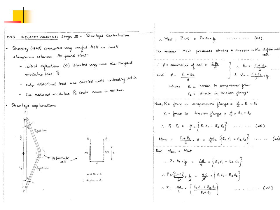
For 50 years, engineers were faced with the dilemma that the reduced modulus theory is correct, but the experimental data was closer to the tangent modulus theory. How to resolve? Shanley eventually resolved this dilemma in He conducted very careful experiments on small aluminum columns. He found that lateral deflection started very near the theoretical tangent modulus load and the load capacity increased with increasing lateral deflections. The column axial load capacity never reached the calculated reduced or double modulus load. Shanley developed a column model to explain the observed phenomenon

Column Inelastic Buckling
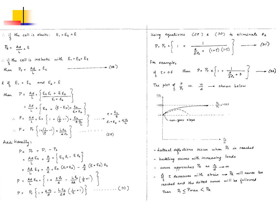
Three different theories Tangent modulus Reduced modulus Shanley model Tangent modulus theory assumes Perfectly straight column Ends are pinned Small deformations No strain reversal during buckling P dP/dv=0 v Elastic buckling analysis Slope is zero at buckling P=0 with increasing v PT

Tangent modulus theory
Assumes that the column buckles at the tangent modulus load such that there is an increase in P (axial force) and M (moment). The axial strain increases everywhere and there is no strain reversal. PT Strain and stress state just before buckling T T=PT/A Strain and stress state just after buckling Mx - Pv = 0 T T v PT Mx v T T=ETT Curvature =  = slope of strain diagram

Tangent modulus theory
Deriving the equation of equilibrium The equation Mx- PTv=0 becomes -ETIxv” - PTv=0 Solution is PT= 2ETIx/L2

Example - Aluminum columns
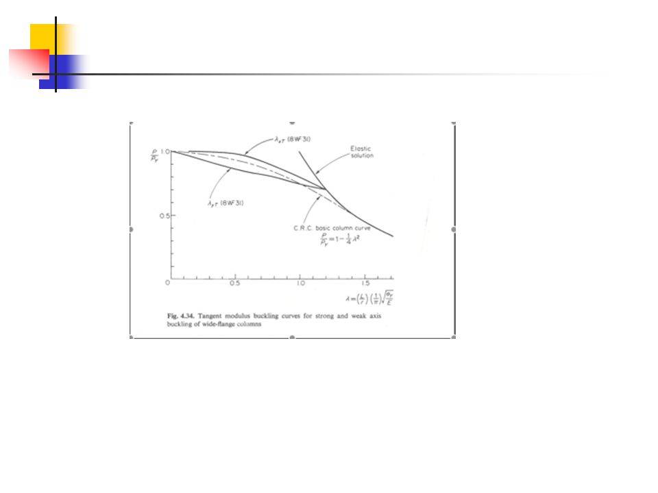
Consider an aluminum column with Ramberg-Osgood stress-strain curve

Tangent Modulus Buckling

x y b d Consider a rectangular section with a simple residual stress distribution Assume that the steel material has elastic-plastic stress-strain  curve. Assume simply supported end conditions Assume triangular distribution for residual stresses rc rc rt y y y/b  y y E 

One major constrain on residual stresses is that they must be such that Residual stresses are produced by uneven cooling but no load is present

b Response will be such that - elastic behavior when x d y b b x y Y Y Y/b

b b x y

Tangent modulus buckling - Numerical
Discretize the cross-section into fibers Think about the discretization. Do you need the flange To be discretized along the length and width? 1 Centroidal axis Afib yfib For each fiber, save the area of fiber (Afib), the distances from the centroid yfib and xfib, Ix-fib and Iy-fib the fiber number in the matrix. 2 Discretize residual stress distribution 3 Calculate residual stress (r-fib) each fiber 4 Check that sum(r-fib Afib)for Section = zero 5

Tangent Modulus Buckling - Numerical
Calculate the critical (KL)X and (KL)Y for the  (KL)X-cr =  sqrt [(EI)Tx/P] (KL)y-cr =  sqrt [(EI)Ty/P] 14 Calculate effective residual strain (r) for each fiber r=r/E 6 Calculate the tangent (EI)TX and (EI)TY for the  (EI)TX = sum(ET-fib{yfib2 Afib+Ix-fib}) (EI)Ty = sum(ET-fib{xfib2 Afib+ Iy-fib}) 13 Assume centroidal strain  7 Calculate average stress =  = P/A 12 Calculate total strain for each fiber tot=+r 8 Calculate Axial Force = P Sum (fibAfib) 11 Assume a material stress-strain curve for each fiber Calculate stress in each fiber fib 10 9

Tangent modulus buckling - numerical

Tangent Modulus Buckling - numerical

Tangent Modulus Buckling - Numerical

ELASTIC BUCKLING OF BEAMS
Going back to the original three second-order differential equations: 1 (MTX+MBX) (MTY+MBY) 2 3

Consider the case of a beam subjected to uniaxial bending only: because most steel structures have beams in uniaxial bending Beams under biaxial bending do not undergo elastic buckling P=0; MTY=MBY=0 The three equations simplify to: Equation (1) is an uncoupled differential equation describing in-plane bending behavior caused by MTX and MBX 1 (-f) 2 3

Equations (2) and (3) are coupled equations in u and f – that describe the lateral bending and torsional behavior of the beam. In fact they define the lateral torsional buckling of the beam. The beam must satisfy all three equations (1, 2, and 3). Hence, beam in-plane bending will occur UNTIL the lateral torsional buckling moment is reached, when it will take over. Consider the case of uniform moment (Mo) causing compression in the top flange. This will mean that -MBX = MTX = Mo

For this case, the differential equations (2 and 3) will become:

Assume simply supported boundary conditions for the beam:

CE 579: STRUCTRAL STABILITY AND DESIGN

Similar presentations

Presentation on theme: "CE 579: STRUCTRAL STABILITY AND DESIGN"— Presentation transcript:

Similar presentations

About project

Feedback

Log in

Auth with social network:

CE 579: STRUCTRAL STABILITY AND DESIGN

Similar presentations

Presentation on theme: "CE 579: STRUCTRAL STABILITY AND DESIGN"— Presentation transcript:

Similar presentations

About project

Feedback