1. DCSP-5: Noise Jianfeng Feng Department of Computer Science Warwick Univ., UK Jianfeng.feng@warwick.ac.uk http://www.dcs.warwick.ac.uk/~feng/dcsp.html

2. Assignment:2015 Q1: you should be able to do it after last week seminar Q2: need a bit reading (my lecture notes) Q3: standard Q4: standard

3. Assignment:2015 Q5: standard Q6: standard Q7: after today’s lecture Q8: load jazz, plot soundsc load Tunejazz plot load NoiseJazz plot

4. Recap Fourier Transform for a periodic signal { sim(n  t), cos(n  t)} For general function case,

5. Recap : this is all you have to remember (know)? Fourier Transform for a periodic signal { sim(n  t), cos(n  t)} For general function case,

6. Can you do FT for cos(2  t)? Dirac delta function

7. For example, take F=0 in the equation above, we have It makes no sense !!!!

8. Dirac delta function: A photo with the highest IQ (15 NL) Dirac Einstein Shordiger Pauli Heisenberg Langevin De Boer Bone Lorentz M Curie Planck Compton Ehrenfest Bragg Debije

9. Dirac Einstein Shordiger Pauli Heisenberg Langevin De Boer Bone Lorentz M Curie Planck Compton Ehrenfest Bragg Debije Dirac delta function: A photo with the highest IQ (15 NL)

10. Dirac delta function The (digital) delta function, for a given n 0 n 0 =0 here  (t)

11. Dirac delta function The (digital) delta function, for a given n 0 Dirac delta function  (x) (you could find a nice movie in Wiki); n 0 =0 here  (t)

12. Dirac delta function Dirac delta function  (x); The FT of cos(2  t) is -1 0 1Frequency

13. A final note (in exam or future) Fourier Transform for a periodic signal { sim(n  t), cos(n  t)} For general function case （ it is true, but need a bit further work),

14. Summary Will come back to it soon (numerical) This trick (FT) has changed our life and will continue to do so

15. This Week’s Summary Noise Information Theory

16. Noise in communication systems: probability and random signals I = imread('peppers.png'); imshow(I); noise = 1*randn(size(I)); Noisy = imadd(I,im2uint8(noise)); imshow(Noisy); Noise

17. Noise in communication systems: probability and random signals I = imread('peppers.png'); imshow(I); noise = 1*randn(size(I)); Noisy = imadd(I,im2uint8(noise)); imshow(Noisy); Noise

18. Noise is a random signal (in general). By this we mean that we cannot predict its value. We can only make statements about the probability of it taking a particular value Noise

19. The probability density function (pdf) p(x) of a random variable x is the probability that x takes a value between x 0 and x 0 +  x. We write this as follows: p(x 0 )  x =P(x 0 <x< x 0 +  x) pdf [x 0 x 0 +  x] P(x)

20. Probability that x will take a value lying between x 1 and x 2 is The probability is unity. Thus pdf

21. Mentally Inadequate 23% Low Intelligence 13.6% Average 34.1% Above Average 34.1% High Intelligence 13.6% Superior Intelligence 2.1% Exceptionally Gifted 0.13% IQ distribution

22. A density satifying the equation is termed normalized. The cumulative distribution function (CDF) F(x) is the probability x is less than x 0 My IQ is above 85% (F(my IQ)=85%). pdf

23. From the rules of integration: P(x 1 <x<x 2 ) = P(x 2 ) --P(x 1 ) pdf has two classes: continuous and discrete pdf

24. Continuous distribution An example of a continuous distribution is the Normal, or Gaussian distribution: where ,  is the mean and standard variation value of p(x). The constant term ensures that the distribution is normalized.

25. Continuous distribution. This expression is important as many actually occurring noise source can be described by it, i.e. white noise or coloured noise.

26. Generating f(x) from matlab X=randn(1,1000); Plot(x); X[1], x[2], …. X[1000], Each x[i] is independent Histogram

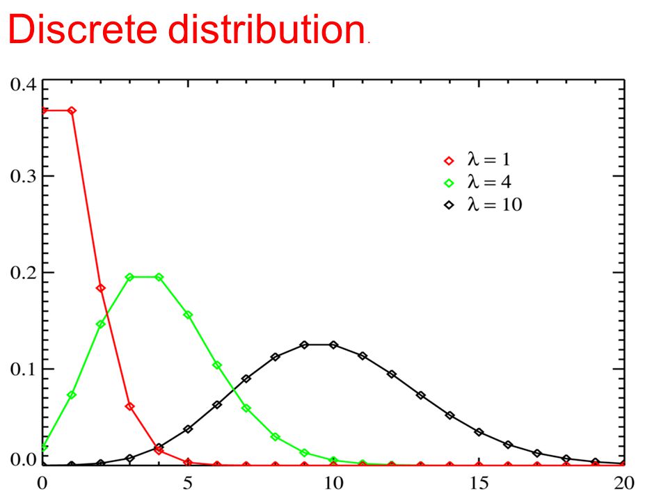
27. If a random variable can only take discrete value, its pdf takes the forms of lines. An example of a discrete distribution is the Poisson distribution Discrete distribution.

29. We cannot predicate value a random variable We can introduce measures that summarise what we expect to happen on average. The two most important measures are the mean (or expectation) and the standard deviation. The mean of a random variable x is defined to be Mean and variance

30. In the examples above we have assumed that the mean of the Gaussian distribution to be 0, the mean of the Poisson distribution is found to be.

31. The mean of a distribution is, in common sense, the average value. Can be estimated from data Assume that {x 1, x 2, x 3, …,x N } are sampled from a distribution Law of Large Numbers: EX ~ (x 1 +x 2 +…+x N )/N Mean and variance

32. The more data we have, the more accurate we can estimate the mean (x 1 +x 2 +…+x N )/N against N for randn(1,N) mean

33. The variance is defined as The variance  is defined to be The square root of the variance is called standard deviation. Again, it can be estimated from data Mean and variance

34. The standard deviation is a measure of the spread of the probability distribution around the mean. A small standard deviation means the distribution are close to the mean. A large value indicates a wide range of possible outcomes. The Gaussian distribution contains the standard deviation within its definition (  ) Mean and variance

35. Communication signals can be modelled as a zero-mean, Gaussian random variable. This means that its amplitude at a particular time has a PDF given by Eq. above. The statement that noise is zero mean says that, on average, the noise signal takes the values zero. Mean and variance

36. http://en.wikipedia.org/wiki/Nations_and_intelligence Mean and variance

37. Einstein’s IQ Mentally Inadequate 23% Low Intelligence 13.6% Average 34.1% Above Average 34.1% High Intelligence 13.6% Superior Intelligence 2.1% Exceptionally Gifted 0.13% Einstein’s IQ=160+ What about yours?

38. Signal to noise ratio is an important quantity in determining the performance of a communication channel. The noise power referred to in the definition is the mean noise power. It can therefore be rewritten as SNR= 10 log 10 ( S /  2 ) SNR

39. Correlation or covariance Cov(X,Y) = E(X-EX)(Y-EY) correlation coefficient is normalized covariance Coef(X,Y) = E(X-EX)(Y-EY) / [  (X)  (Y)] Positive correlation, Negative correlation No correlation (independent)

40. Stochastic process = signal A stochastic process is a collection of random variables x[n], for each fixed [n], it is a random variable Signal is a typical stochastic process To understand how x[n] evolves with n, we will look at auto-correlation function (ACF) ACF is the correlation between k steps

41. Stochastic process >> clear all close all n=200; for i=1:10 x(i)=randn(1,1); y(i)=x(i); end for i=1:n-10 y(i+10)=randn(1,1); x(i+10)=.8*x(i)+y(i+10); end plot(xcorr(x)/max(xcorr(x))); hold on plot(xcorr(y)/max(xcorr(y)),'r') two signals are generated: y (red) is simply randn(1,200) x (blue) is generated x[i+10]=.8*x[i] + y[i+10] For y, we have  (0)=1,  (n)=0, if n is not 0 : having no memory For x, we have  (0)=1, and  (n) is not zero, for some n: having memory

42. white noise w[n] White noise is a random process we can not predict at all (independent of history) In other words, it is the most ‘violent’ noise White noise draws its name from white light which will become clear in the next few lectures

43. The most ‘noisy’ noise is a white noise since its autocorrelation is zero, i.e. corr(w[n], w[m])=0 when Otherwise, we called it colour noise since we can predict some outcome of w[n], given w[m], m<n white noise w[n]

44. Why do we love Gaussian? Sweety Gaussian

45. + = Sweety Gaussian A linear combination of two Gaussian random variables is Gaussian again For example, given two independent Gaussian variable X and Y with mean zero aX+bY is a Gaussian variable with mean zero and variance a 2  (X)+b 2  (Y) This is very rare (the only one in continuous distribution) but extremely useful: panda in the family of all distributions Yes, I am junior Gaussian Herr Gauss + Frau Gauss = Juenge Gauss

46. DCSP-6: Information Theory Jianfeng Feng Department of Computer Science Warwick Univ., UK Jianfeng.feng@warwick.ac.uk http://www.dcs.warwick.ac.uk/~feng/dcsp.html

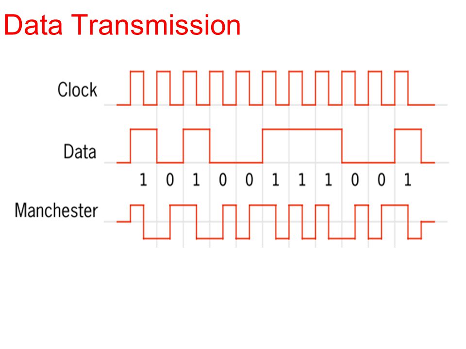
47. Data Transmission

48. How to deal with noise? How to transmit signals? Data Transmission

50. Transform I Fourier Transform ASK (AM), FSK(FM), and PSK (skipped, but common knowledge) Noise Signal Transmission Data Transmission

51. Data transmission: Shannon Information and Coding: Information theory, coding of information for efficiency and error protection; Today

52. Information and coding theory Information theory is concerned with description of information sources representation of the information from a source (coding), transmission of this information over channel.

53. Information and coding theory The best example how a deep mathematical theory could be successfully applied to solving engineering problems. Information and coding theory

54. Information theory is a discipline in applied mathematics involving the quantification of data with the goal of enabling as much data as possible to be reliably stored on a medium and/or communicated over a channel. Information and coding theory

55. The measure of data, known as information entropy, is usually expressed by the average number of bits needed for storage or communication. Information and coding theory

56. The field is at the crossroads of Information and coding theory mathematics, statistics, computer science, physics, neurobiology, electrical engineering.

57. Impact has been crucial to success of voyager missions to deep space, invention of the CD, feasibility of mobile phones, development of the Internet, the study of linguistics and of human perception, understanding of black holes, and numerous other fields. Information and coding theory

58. Founded in 1948 by Claude Shannon in his seminal work A Mathematical Theory of Communication Information and coding theory

59. The ‘bible’ paper: cited more than 60,000

60. The most fundamental results of this theory are 1. Shannon's source coding theorem the number of bits needed to represent the result of an uncertain event is given by its entropy; 2. Shannon's noisy-channel coding theorem reliable communication is possible over noisy channels if the rate of communication is below a certain threshold called the channel capacity. The channel capacity can be approached by using appropriate encoding and decoding systems. Information and coding theory

61. The most fundamental results of this theory are 1. Shannon's source coding theorem the number of bits needed to represent the result of an uncertain event is given by its entropy; 2. Shannon's noisy-channel coding theorem reliable communication is possible over noisy channels if the rate of communication is below a certain threshold called the channel capacity. The channel capacity can be approached by using appropriate encoding and decoding systems. Information and coding theory

62. Consider to predict the activity of Prime minister tomorrow. This prediction is an information source. Information and coding theory

63. Consider to predict the activity of Prime Minister tomorrow. This prediction is an information source X. The information source X ={O, R} has two outcomes: He will be in his office (O), he will be naked and run 10 miles in London (R). Information and coding theory

64. Clearly, the outcome of 'in office' contains little information; it is a highly probable outcome. The outcome 'naked run', however contains considerable information; it is a highly improbable event. Information and coding theory

65. An information source is a probability distribution, i.e. a set of probabilities assigned to a set of outcomes (events). This reflects the fact that the information contained in an outcome is determined not only by the outcome, but by how uncertain it is. An almost certain outcome contains little information. A measure of the information contained in an outcome was introduced by Hartley in 1927. Information and coding theory

66. Defined the information contained in an outcome x i in x={x 1, x 2,…,x n } I(x i ) = - log 2 p(x i ) Information

67. The definition above also satisfies the requirement that the total information in in dependent events should add. Clearly, our prime minister prediction for two days contain twice as much information as for one day. Information

68. The definition above also satisfies the requirement that the total information in in dependent events should add. Clearly, our prime minister prediction for two days contain twice as much information as for one day X={OO, OR, RO, RR}. For two independent outcomes x i and x j, I(x i and x j ) = - log 2 P(x i and x j ) = - log 2 P(x i ) P(x j ) = - log 2 P(x i ) - log 2 P(x j ) Information

69. The measure entropy H(X) defines the information content of the source X as a whole. It is the mean information provided by the source. We have H(X)=  i P(x i ) I(x i ) = -  i P(x i ) log 2 P(x i ) A binary symmetric source (BSS) is a source with two outputs whose probabilities are p and 1-p respectively. Entropy

70. The prime minister discussed is a BSS. The entropy of the BBS source is H(X) = -p log 2 p - (1-p) log 2 (1-p) Entropy

71. . When one outcome is certain, so is the other, and the entropy is zero. As p increases, so too does the entropy, until it reaches a maximum when p = 1-p = 0.5. When p is greater than 0.5, the curve declines symmetrically to zero, reached when p=1. Entropy

72. Next Week Application of Entropy in coding Minimal length coding

73. We conclude that the average information in BSS is maximised when both outcomes are equally likely. Entropy is measuring the average uncertainty of the source. (The term entropy is borrowed from thermodynamics. There too it is a measure of the uncertainly of disorder of a system). Shannon: My greatest concern was what to call it. I thought of calling it ‘information’, but the word was overly used, so I decided to call it ‘uncertainty’. When I discussed it with John von Neumann, he had a better idea.John von Neumann Von Neumann told me, ‘You should call it entropy, for two reasons. In the first place your uncertainty function has been used in statistical mechanics under that name, so it already has a name. In the second place, and more important, nobody knows what entropy really is, so in a debate you will always have the advantage. Entropy

74. In Physics: thermodynamics The arrow of time (Wiki) Entropy is the only quantity in the physical sciences that seems to imply a particular direction of progress, sometimes called an arrow of time.arrow of time. As time progresses, the second law of thermodynamics states that the entropy of an isolated systems never decreases Hence, from this perspective, entropy measurement is thought of as a kind of clock

75. Entropy