4. 3-1 Introduction Experiment Random Random experiment

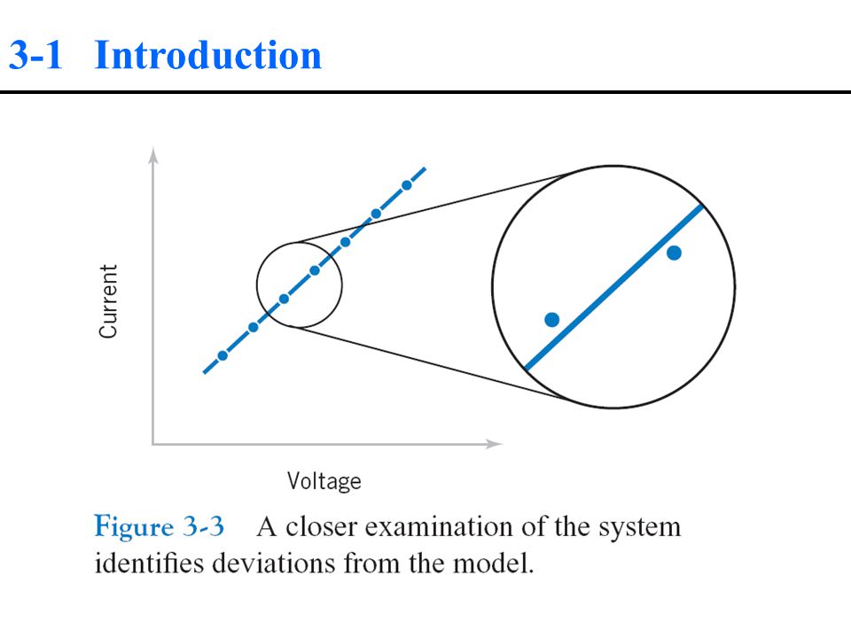
5. 3-1 Introduction

9. 3-2 Random Variables In an experiment, a measurement is usually denoted by a variable such as X. In a random experiment, a variable whose measured value can change (from one replicate of the experiment to another) is referred to as a random variable.

10. 3-2 Random Variables

11. 3-3 Probability Used to quantify likelihood or chance Used to represent risk or uncertainty in engineering applications Can be interpreted as our degree of belief or relative frequency

12. 3-3 Probability Probability statements describe the likelihood that particular values occur. The likelihood is quantified by assigning a number from the interval [0, 1] to the set of values (or a percentage from 0 to 100%). Higher numbers indicate that the set of values is more likely.

13. 3-3 Probability A probability is usually expressed in terms of a random variable. For the part length example, X denotes the part length and the probability statement can be written in either of the following forms Both equations state that the probability that the random variable X assumes a value in [10.8, 11.2] is 0.25.

14. 3-3 Probability Complement of an Event Given a set E, the complement of E is the set of elements that are not in E. The complement is denoted as E ’. Mutually Exclusive Events The sets E 1, E 2,...,E k are mutually exclusive if the intersection of any pair is empty. That is, each element is in one and only one of the sets E 1, E 2,...,E k.

15. 3-3 Probability Probability Properties

16. 3-3 Probability Events A measured value is not always obtained from an experiment. Sometimes, the result is only classified (into one of several possible categories). These categories are often referred to as events. Illustrations The current measurement might only be recorded as low, medium, or high; a manufactured electronic component might be classified only as defective or not; and either a message is sent through a network or not.

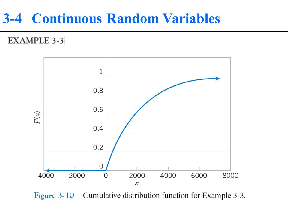
17. 3-4 Continuous Random Variables 3-4.1 Probability Density Function The probability distribution or simply distribution of a random variable X is a description of the set of the probabilities associated with the possible values for X.

18. 3-4 Continuous Random Variables 3-4.1 Probability Density Function

19. 3-4 Continuous Random Variables 3-4.1 Probability Density Function

20. 3-4 Continuous Random Variables 3-4.1 Probability Density Function

21. 3-4 Continuous Random Variables 3-4.1 Probability Density Function

22. 3-4 Continuous Random Variables

24. 3-4.2 Cumulative Distribution Function

25. 3-4 Continuous Random Variables

28. 3-4.3 Mean and Variance

29. 3-4 Continuous Random Variables

30. 3-5 Important Continuous Distributions 3-5.1 Normal Distribution Undoubtedly, the most widely used model for the distribution of a random variable is a normal distribution. Central limit theorem Gaussian distribution

31. 3-5 Important Continuous Distributions 3-5.1 Normal Distribution

32. 3-5 Important Continuous Distributions 3-5.1 Normal Distribution

33. 3-5 Important Continuous Distributions

34. 3-5.1 Normal Distribution

35. 3-5 Important Continuous Distributions 3-5.1 Normal Distribution

36. 3-5 Important Continuous Distributions 3-5.1 Normal Distribution

37. 3-5 Important Continuous Distributions

38. 3-5.1 Normal Distribution

39. 3-5 Important Continuous Distributions 3-5.1 Normal Distribution

40. 3-5 Important Continuous Distributions

42. 3-5.2 Lognormal Distribution

43. 3-5 Important Continuous Distributions 3-5.2 Lognormal Distribution

44. 3-5 Important Continuous Distributions 3-5.3 Gamma Distribution

45. 3-5 Important Continuous Distributions 3-5.3 Gamma Distribution

46. 3-5 Important Continuous Distributions 3-5.3 Gamma Distribution

47. 3-5 Important Continuous Distributions 3-5.4 Weibull Distribution

48. 3-5 Important Continuous Distributions 3-5.4 Weibull Distribution

49. 3-5 Important Continuous Distributions 3-5.4 Weibull Distribution

50. 3-6 Probability Plots 3-6.1 Normal Probability Plots How do we know if a normal distribution is a reasonable model for data? Probability plotting is a graphical method for determining whether sample data conform to a hypothesized distribution based on a subjective visual examination of the data. Probability plotting typically uses special graph paper, known as probability paper, that has been designed for the hypothesized distribution. Probability paper is widely available for the normal, lognormal, Weibull, and various chi- square and gamma distributions.

51. 3-6 Probability Plots 3-6.1 Normal Probability Plots

52. 3-6 Probability Plots 3-6.1 Normal Probability Plots

53. 3-6 Probability Plots 3-6.2 Other Probability Plots

54. 3-6 Probability Plots 3-6.2 Other Probability Plots

55. 3-6 Probability Plots 3-6.2 Other Probability Plots

56. 3-6 Probability Plots 3-6.2 Other Probability Plots

57. 3-7 Discrete Random Variables Only measurements at discrete points are possible

58. 3-7 Discrete Random Variables 3-7.1 Probability Mass Function

59. 3-7 Discrete Random Variables 3-7.1 Probability Mass Function

60. 3-7 Discrete Random Variables 3-7.1 Probability Mass Function

61. 3-7 Discrete Random Variables 3-7.2 Cumulative Distribution Function

62. 3-7 Discrete Random Variables 3-7.2 Cumulative Distribution Function

63. 3-7 Discrete Random Variables 3-7.3 Mean and Variance

64. 3-7 Discrete Random Variables 3-7.3 Mean and Variance

65. 3-7 Discrete Random Variables 3-7.3 Mean and Variance

66. 3-8 Binomial Distribution A trial with only two possible outcomes is used so frequently as a building block of a random experiment that it is called a Bernoulli trial. It is usually assumed that the trials that constitute the random experiment are independent. This implies that the outcome from one trial has no effect on the outcome to be obtained from any other trial. Furthermore, it is often reasonable to assume that the probability of a success on each trial is constant.

67. 3-8 Binomial Distribution Consider the following random experiments and random variables. Flip a coin 10 times. Let X = the number of heads obtained. Of all bits transmitted through a digital transmission channel, 10% are received in error. Let X = the number of bits in error in the next 4 bits transmitted. Do they meet the following criteria: 1. Does the experiment consist of Bernoulli trials? 2.Are the trials that constitute the random experiment are independent? 3.Is probability of a success on each trial is constant?

68. 3-8 Binomial Distribution

71. 3-9 Poisson Process

72. 3-9.1 Poisson Distribution

73. 3-9 Poisson Process 3-9.1 Poisson Distribution

74. 3-9 Poisson Process 3-9.1 Poisson Distribution

75. 3-9 Poisson Process 3-9.1 Poisson Distribution

76. 3-9 Poisson Process 3-9.1 Poisson Distribution

77. 3-9 Poisson Process 3-9.2 Exponential Distribution The discussion of the Poisson distribution defined a random variable to be the number of flaws along a length of copper wire. The distance between flaws is another random variable that is often of interest. Let the random variable X denote the length from any starting point on the wire until a flaw is detected. As you might expect, the distribution of X can be obtained from knowledge of the distribution of the number of flaws. The key to the relationship is the following concept: The distance to the first flaw exceeds 3 millimeters if and only if there are no flaws within a length of 3 millimeters—simple, but sufficient for an analysis of the distribution of X.

78. 3-9 Poisson Process 3-9.2 Exponential Distribution

79. 3-9 Poisson Process 3-9.2 Exponential Distribution

80. 3-9 Poisson Process 3-9.2 Exponential Distribution

81. 3-9 Poisson Process 3-9.2 Exponential Distribution The exponential distribution is often used in reliability studies as the model for the time until failure of a device. For example, the lifetime of a semiconductor chip might be modeled as an exponential random variable with a mean of 40,000 hours. The lack of memory property of the exponential distribution implies that the device does not wear out. The lifetime of a device with failures caused by random shocks might be appropriately modeled as an exponential random variable. However, the lifetime of a device that suffers slow mechanical wear, such as bearing wear, is better modeled by a distribution that does not lack memory.

82. 3-10Normal Approximation to the Binomial and Poisson Distributions Normal Approximation to the Binomial

83. 3-10Normal Approximation to the Binomial and Poisson Distributions Normal Approximation to the Binomial

84. 3-10Normal Approximation to the Binomial and Poisson Distributions Normal Approximation to the Binomial

85. 3-10Normal Approximation to the Binomial and Poisson Distributions Normal Approximation to the Poisson

86. 3-11More Than One Random Variable and Independence 3-11.1 Joint Distributions

87. 3-11More Than One Random Variable and Independence 3-11.1 Joint Distributions

88. 3-11More Than One Random Variable and Independence 3-11.1 Joint Distributions

89. 3-11More Than One Random Variable and Independence 3-11.1 Joint Distributions

90. 3-11More Than One Random Variable and Independence 3-11.2 Independence

91. 3-11More Than One Random Variable and Independence 3-11.2 Independence

92. 3-11More Than One Random Variable and Independence 3-11.2 Independence

93. 3-11More Than One Random Variable and Independence 3-11.2 Independence

94. 3-12Functions of Random Variables

95. 3-12.1 Linear Combinations of Independent Random Variables

96. 3-12Functions of Random Variables 3-12.1 Linear Combinations of Independent Random Variables

97. 3-12Functions of Random Variables 3-12.1 Linear Combinations of Independent Random Variables

98. 3-12Functions of Random Variables 3-12.2 What If the Random Variables Are Not Independent?

99. 3-12Functions of Random Variables 3-12.2 What If the Random Variables Are Not Independent?

100. 3-12Functions of Random Variables 3-12.3 What If the Function Is Nonlinear?

101. 3-12Functions of Random Variables 3-12.3 What If the Function Is Nonlinear?

102. 3-12Functions of Random Variables 3-12.3 What If the Function Is Nonlinear?

103. 3-13Random Samples, Statistics, and The Central Limit Theorem

104. 3-13Random Samples, Statistics, and The Central Limit Theorem Central Limit Theorem

105. 3-13Random Samples, Statistics, and The Central Limit Theorem

106. 3-13Random Samples, Statistics, and The Central Limit Theorem

107. 3-13Random Samples, Statistics, and The Central Limit Theorem