1. DCSP-2: Fourier Transform I Jianfeng Feng Department of Computer Science Warwick Univ., UK Jianfeng.feng@warwick.ac.uk http://www.dcs.warwick.ac.uk/~feng/dcsp.html

2. The range of frequencies occupied by the signal is called its bandwidth.

3. The ADC process is governed by an important law. Nyquist-Shannon Theorem (will be discussed in Chapter 3) An analogue signal of bandwidth B can be completely recreated from its sampled form provided its sampled at a rate equal to at least twice it bandwidth. That is S >= 2 B

4. Example, a speech signal has an approximate bandwidth of 4KHz. If this is sampled by an 8-bit ADC at the Nyquist sampling, the bit rate R is R=8 bits x 2 B=6400 b/s

5. The relationship between information, bandwidth and noise The most important question associated with a communication channel is the maximum rate at which it can transfer information. Is there a limit on the number of levels? The limit is set by the presence of noise. If we continue to subdivide the magnitude of the changes into ever decreasing intervals, we reach a point where we cannot distinguish the individual levels because of the presence of noise.

6. Noise therefore places a limit on the maximum rate at which we can transfer information Obviously, what really matters is the signal to noise ratio (SNR). This is defined by the ratio signal power S to noise power N, and is often expressed in deciBels (dB): SNR=10 log 10 (S/N) dB

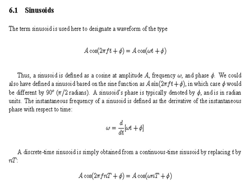
7. Most signal carried by communication channels are modulated forms of sine waves. A sine wave is described mathematically by the expression s(t)=A cos ( t The quantities A,, are termed the amplitude, frequency and phase of the sine wave.

8. When referring to measurements of amplitude it is usual to consider the ratio of the squares of A1 (measured amplitude) and A0 (reference amplitude). This is because in most applications power is proportional to the square of amplitude. Thus the following definition is used: SNR=10 log 10 (A1/A0)= dB

9. Noise sources Input noise is common in low frequency circuits and arises from electric fields generated by electrical switching. It appears as bursts at the receiver, and when present can have a catastrophic effect due to its large power. Other peoples signals can generate noise: cross-talk is the term give to the pick-up of radiated signals from adjacent cabling.

10. Noise sources When radio links are used, interference from other transmitters can be problematic. Thermal noise is always present. It is due to the random motion of electric charges present in all media. It can be generated externally, or internally at the receiver.

11. There is a theoretical maximum to the rate at which information passes error free over the channel. This maximum is called the channel capacity, C. The famous Hartley-Shannon Law states that the channel capacity, C (we will discuss in details in Chapter 3) is given by C=B log_2(1+(S/N)) b/s

12. For example, a 10kHz channel operating at a SNR of 15dB has a theoretical maximum information rate of 10000 log 2 (31.623)=49828 b/s. The theorem makes no statement as to how the channel capacity is achieved. In fact, in practice channels only approach this limit. The task of providing high channel efficiency is the goal of coding techniques.

13. Two basic laws Nyquist-Shannon sampling theorem Hartley-Shannon Law (channel capacity)

14. Analog signal sampling quantized coding channel receiver bandwidth

15. Communication Techniques Time, frequency and bandwidth (Fourier Transform)

16. Communication Techniques Time, frequency and bandwidth We can describe this signal in two ways. One way is to describe its evolution in time domain, as in the equation above. The other way is to describe its frequency content, in frequency domain. The cosine wave, s(t), has a single frequency, =2 /T where T is the period i.e. S(t+T)=s(t).

17. This representation is quite general. In fact we have the following theorem due to Fourier. Any signal x(t) of period T can be represented as the sum of a set of cosinusoidal and sinusoidal waves of different frequencies and phases.

18. In mathematics, the continuous Fourier transform is one of the specific forms of Fourier analysis. As such, it transforms one function into another, which is called the frequency domain representation of the original function (which is often a function in the time- domain). In this specific case, both domains are continuous and unbounded. The term Fourier transform can refer to either the frequency domain representation of a function or to the process/formula that "transforms" one function into the other.