1. Particle Filters++ TexPoint fonts used in EMF.
Pieter Abbeel
UC Berkeley EECS
Many slides adapted from Thrun, Burgard and Fox, Probabilistic Robotics
TexPoint fonts used in EMF.
Read the TexPoint manual before you delete this box.: AAAAAAAAAAAAA

2. Sequential Importance Resampling (SIR) Particle Filter
Algorithm particle_filter( St-1, ut , zt):
For Generate new samples
Sample index j(i) from the discrete distribution given by wt-1
Sample from
Compute importance weight
Update normalization factor
Insert
For
Normalize weights
Return St

3. Outline Improved Sampling
Issue with vanilla particle filter when noise dominated by motion model
Importance Sampling
Optimal Proposal
Examples
Resampling
Particle Deprivation
Noise-free Sensors
Adapting Number of Particles: KLD Sampling

4. Noise Dominated by Motion Model
[Grisetti, Stachniss, Burgard, T-RO2006]
 Most particles get (near) zero weights and are lost.

5. Importance Sampling
Theoretical justification: for any function f we have:
f could be: whether a grid cell is occupied or not, whether the position of a robot is within 5cm of some (x,y), etc.

6. Importance Sampling Task: sample from density p(.) Solution:
sample from “proposal density” ¼(.)
Weight each sample x(i) by p(x(i)) / ¼(x(i))
E.g.:
Requirement: if ¼(x) = 0 then p(x) = 0. p

7. Particle Filters Revisited
Algorithm particle_filter( St-1, ut , zt):
For Generate new samples
Sample index j(i) from the discrete distribution given by wt-1
Sample from
Compute importance weight
Update normalization factor
Insert
For
Normalize weights
Return St

8. Optimal Sequential Proposal ¼(.)
Applying Bayes rule to the denominator gives:
Substitution and simplification gives

9. Optimal proposal ¼(.) Optimal =  Challenges:
Typically difficult to sample from
Importance weight: typically expensive to compute integral

10. Example 1: ¼(.) = Optimal proposal Nonlinear Gaussian State Space Model
Then:
with
And:

11. Example 2: ¼(.) = Motion Model
 the “standard” particle filter

12. Example 3: Approximating Optimal ¼ for Localization
[Grisetti, Stachniss, Burgard, T-RO2006]
One (not so desirable solution): use smoothed likelihood such that more particles retain a meaningful weight --- BUT information is lost
Better: integrate latest observation z into proposal ¼

13. Example 3: Approximating Optimal ¼ for Localization: Generating One Weighted Sample
Initial guess
Execute scan matching starting from the initial guess , resulting in pose estimate .
Sample K points in region around
Proposal distribution is Gaussian with mean and covariance:
Sample from (approximately optimal) proposal distribution.
Weight =

14. Scan Matching
Compute
E.g., using gradient descent

15. Example 3: Example Particle Distributions
[Grisetti, Stachniss, Burgard, T-RO2006]
Particles generated from the approximately optimal proposal distribution. If using the standard motion model, in all three cases the particle set would have been similar to (c).

16. Resampling
Consider running a particle filter for a system with deterministic dynamics and no sensors
Problem:
While no information is obtained that favors one particle over another, due to resampling some particles will disappear and after running sufficiently long with very high probability all particles will have become identical.
On the surface it might look like the particle filter has uniquely determined the state.
Resampling induces loss of diversity. The variance of the particles decreases, the variance of the particle set as an estimator of the true belief increases.

17. Resampling Solution I Effective sample size: Example:
All weights = 1/N  Effective sample size = N
All weights = 0, except for one weight = 1  Effective sample size = 1
Idea: resample only when effective sampling size is low
Normalized weights

18. Resampling Solution I (ctd)

19. Resampling Solution II: Low Variance Sampling
M = number of particles
r \in [0, 1/M]
Advantages:
More systematic coverage of space of samples
If all samples have same importance weight, no samples are lost
Lower computational complexity

20. Resampling Solution III
Loss of diversity caused by resampling from a discrete distribution
Solution: “regularization”
Consider the particles to represent a continuous density
Sample from the continuous density
E.g., given (1-D) particles
sample from the density:

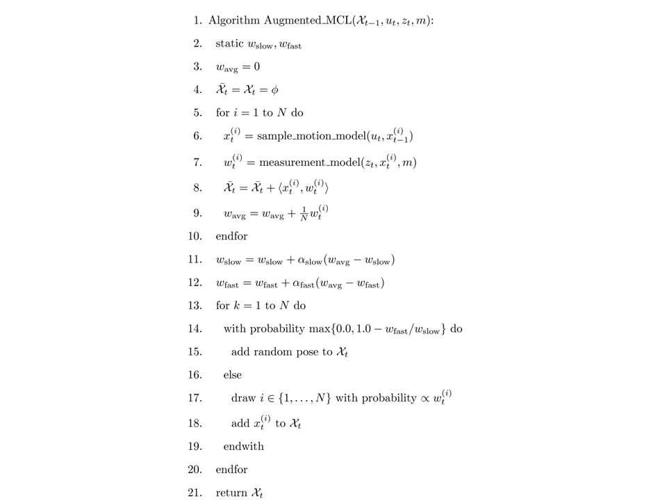
21. Particle Deprivation
= when there are no particles in the vicinity of the correct state
Occurs as the result of the variance in random sampling. An unlucky series of random numbers can wipe out all particles near the true state. This has non-zero probability to happen at each time  will happen eventually.
Popular solution: add a small number of randomly generated particles when resampling.
Advantages: reduces particle deprivation, simplicity.
Con: incorrect posterior estimate even in the limit of infinitely many particles.
Other benefit: initialization at time 0 might not have gotten anything near the true state, and not even near a state that over time could have evolved to be close to true state now; adding random samples will cut out particles that were not very consistent with past evidence anyway, and instead gives a new chance at getting close the true state.

22. Particle Deprivation: How Many Particles to Add?
Simplest: Fixed number.
Better way:
Monitor the probability of sensor measurements
which can be approximated by:
Average estimate over multiple time-steps and compare to typical values when having reasonable state estimates. If low, inject random particles.

24. Noise-free Sensors
Consider a measurement obtained with a noise-free sensor, e.g., a noise-free laser-range finder---issue?
All particles would end up with weight zero, as it is very unlikely to have had a particle matching the measurement exactly.
Solutions:
Artificially inflate amount of noise in sensors
Better proposal distribution (see first section of this set of slides).

25. Adapting Number of Particles: KLD-Sampling
E.g., typically more particles need at the beginning of localization run
Idea:
Partition the state-space
When sampling, keep track of number of bins occupied
Stop sampling when a threshold that depends on the number of occupied bins is reached
If all samples fall in a small number of bins  lower threshold

26. z_{1-\delta}: the upper 1- \delta quantile of the standard normal distribution
\delta = 0.01 and \epsilon = 0.05 works well in practice

27. KLD-sampling

28. KLD-sampling