1. CS 547: Sensing and Planning in Robotics Gaurav S. Sukhatme Computer Science Robotic Embedded Systems Laboratory University of Southern California gaurav@usc.edu http://robotics.usc.edu/~gaurav

2. Bayes Filters: Framework Given: Stream of observations z and action data u: Sensor model P(z|x). Action model P(x|u,x’). Prior probability of the system state P(x). Wanted: Estimate of the state X of a dynamical system. The posterior of the state is also called Belief: Slide courtesy of S. Thrun, D. Fox and W. Burgard

3. Recursive Bayesian Updating Markov assumption: z n is independent of d 1,...,d n-1 if we know x.

4. Markov Assumption Underlying Assumptions Static world Independent noise Perfect model, no approximation errors Slide courtesy of S. Thrun, D. Fox and W. Burgard

5. Recursive Bayesian Updating Action Update

6. Bayes Filter Algorithm 1. Algorithm Bayes_filter( Bel(x),d ): 2. 0 3. If d is a perceptual data item z then 4. For all x do 5. 6. 7. For all x do 8. 9. Else if d is an action data item u then 10. For all x do 11. 12. Return Bel’(x) Slide courtesy of S. Thrun, D. Fox and W. Burgard

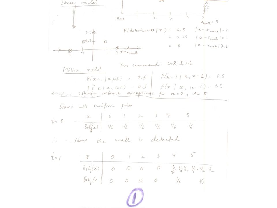
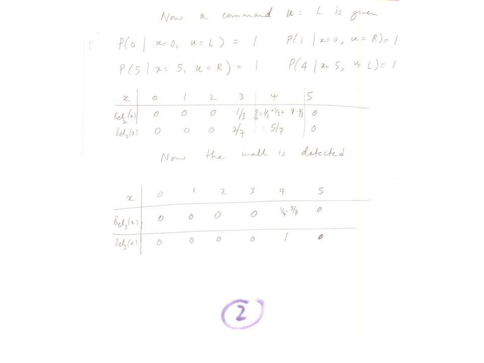
7. 7 Discrete Bayes Filter Algorithm 1. Algorithm Discrete_Bayes_filter( Bel(x),d ): 2. 0 3. If d is a perceptual data item z then 4. For all x do 5. 6. 7. For all x do 8. 9. Else if d is an action data item u then 10. For all x do 11. 12. Return Bel’(x)

8. Bayes Filters Bayes z = observation u = action x = state Markov Total prob. Markov Slide courtesy of S. Thrun, D. Fox and W. Burgard

9. Bayes Filters are Familiar! Kalman filters Particle filters Hidden Markov models Dynamic Bayesian networks Partially Observable Markov Decision Processes (POMDPs) Slide courtesy of S. Thrun, D. Fox and W. Burgard

10. Summary Bayes rule allows us to compute probabilities that are hard to assess otherwise. Under the Markov assumption, recursive Bayesian updating can be used to efficiently combine evidence. Bayes filters are a probabilistic tool for estimating the state of dynamic systems. Slide courtesy of S. Thrun, D. Fox and W. Burgard

15. Prediction Correction Bayes Filter Reminder

16. Gaussians --   Univariate  Multivariate Slide courtesy of S. Thrun, D. Fox and W. Burgard

17. Properties of Gaussians

18. We stay in the “Gaussian world” as long as we start with Gaussians and perform only linear transformations. Multivariate Gaussians

19. Discrete Kalman Filter Estimates the state x of a discrete-time controlled process that is governed by the linear stochastic difference equation with a measurement Slide courtesy of S. Thrun, D. Fox and W. Burgard

20. Components of a Kalman Filter Matrix (nxn) that describes how the state evolves from t to t-1 without controls or noise. Matrix (nxl) that describes how the control u t changes the state from t to t-1. Matrix (kxn) that describes how to map the state x t to an observation z t. Random variables representing the process and measurement noise that are assumed to be independent and normally distributed with covariance R t and Q t respectively. Slide courtesy of S. Thrun, D. Fox and W. Burgard

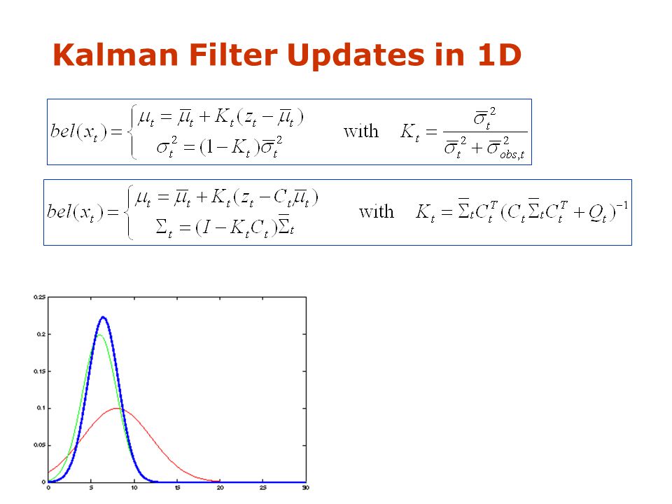
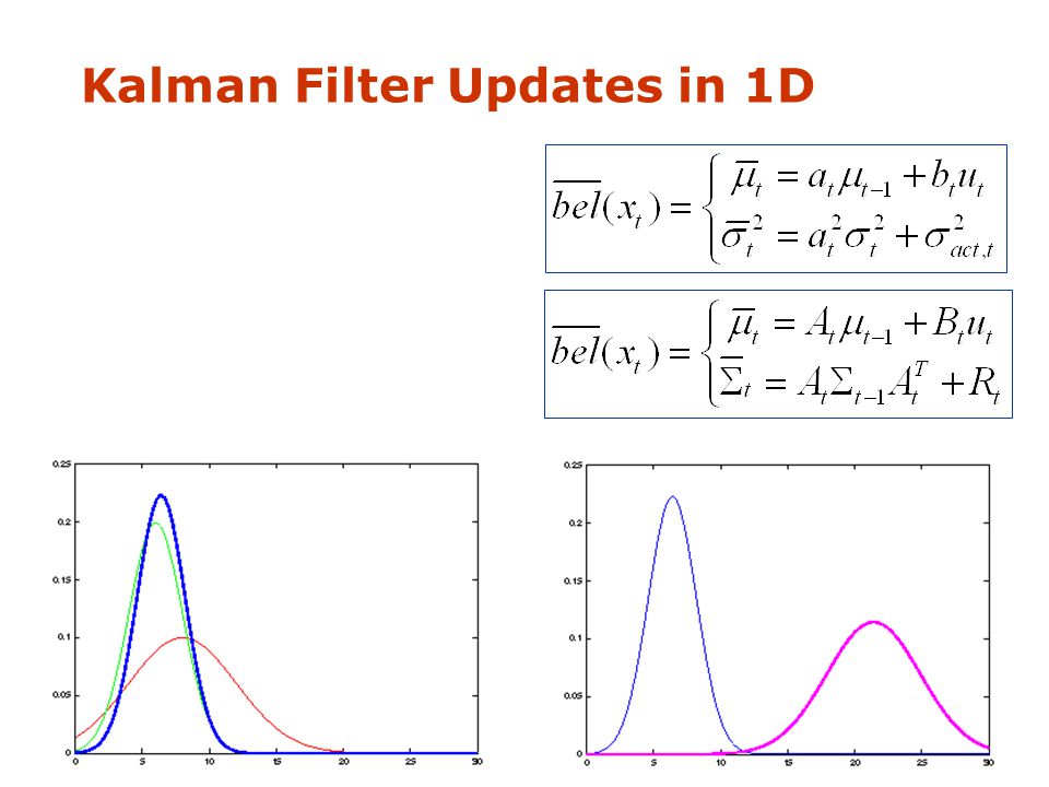
21. Kalman Filter Updates in 1D

24. Kalman Filter Updates

25. Linear Gaussian Systems: Initialization Initial belief is normally distributed:

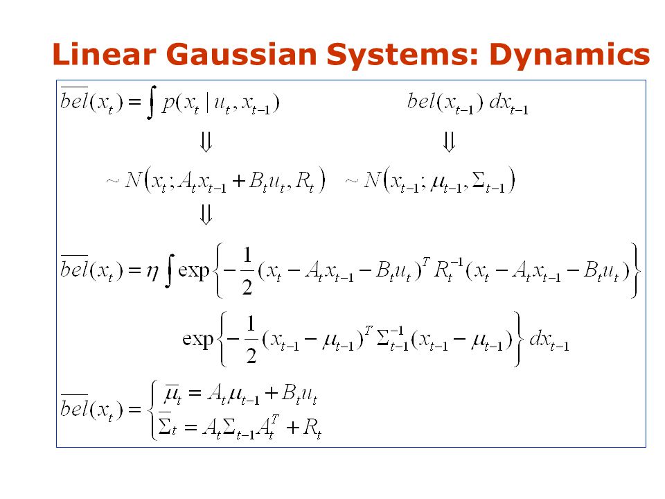
26. Dynamics are linear function of state and control plus additive noise: Linear Gaussian Systems: Dynamics

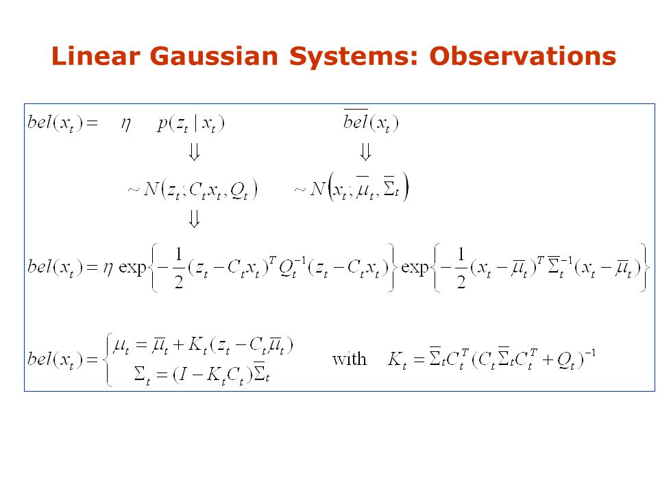
28. Observations are linear function of state plus additive noise: Linear Gaussian Systems: Observations

30. Kalman Filter Algorithm 1. Algorithm Kalman_filter(  t-1,  t-1, u t, z t ): 2. Prediction: 3. 4. 5. Correction: 6. 7. 8. 9. Return  t,  t

31. The Prediction-Correction-Cycle Prediction Slide courtesy of S. Thrun, D. Fox and W. Burgard

32. The Prediction-Correction-Cycle Correction Slide courtesy of S. Thrun, D. Fox and W. Burgard

33. The Prediction-Correction-Cycle Correction Prediction Slide courtesy of S. Thrun, D. Fox and W. Burgard

34. Kalman Filter Summary Highly efficient: Polynomial in measurement dimensionality k and state dimensionality n: O(k 2.376 + n 2 ) Optimal for linear Gaussian systems! Most robotics systems are nonlinear!