1. Andrew Schuh 1, Thomas Lauvaux 2,, Ken Davis 2, Marek Uliasz 1, Dan Cooley 1, Tristram West 3, Liza Diaz 2, Scott Richardson 2, Natasha Miles 2, F. Jay Breidt 1, Arlyn Andrews 4, Kevin Gurney 6, Erandi Lokupitiya 1, Linda Heath 7, James Smith 7, Scott Denning 1, and Stephen M. Ogle 1 Comparing Inversion Results over the Mid-Continental Intensive (MCI) Region 1.Colorado State University, 2. The Pennsylvania State University, 3. Pacific Northwest National Laboratory, 4. NOAA Earth System Research Laboratory, 5. U.S. Forest Service, 6. Arizona State University, 7. U.S. Forest Service We gratefully acknowledge funding support from the National Aeronautics and Space Administration, Earth Sciences Division, to Colorado State University (agreement #NNX08AK08G).

2. Main Goal of MCI Synthesis Compare and reconcile to the extent possible CO 2 fluxes from inventories and atmospheric inversions C CO 2 C Atmospheric Inversions Inventories

3. “Top-down” vs “Bottom-up” Accurately captures all C contributions, whether known or unknown Integrates and mixes signals, thus generally better used at larger spatial scales then inventory Depends on accurate modeling of transport which can be difficult InventoriesAtmospheric Inversions Process based and thus fluxes are “attributable”, good for policy decisions Generally tied to valuable commodities and thus tracked well, e.g. crop production, forest inventory, etc. Generally sampled at point locations and upscaled and thus possibly not as accurate at larger scales

4. Total 2007 NEE (Inventory minus fossil) Note largest sink driven by crop signal over corn belt Largest uncertainty is over non-crop lands, presumably forest driven, on scale of 50% of max sink strength Note human respiration component over Chicago MEA N SD -350gCm -2 yr -1 +350gCm -2 yr -1 +250gCm -2 yr -1 0gCm -2 yr -1 Posters Ogle H-184 Ogle F-129 West G-167

5. CarbonTracker as Baseline

6. Summing over MCI Region

7. CarbonTracker vs MCI Inventory -350gCm -2 yr -1 100gCm -2 yr -1

8. CarbonTracker vs MCI Inventory In general, looks pretty reasonable -350gCm -2 yr -1 100gCm -2 yr -1

9. CarbonTracker vs MCI Inventory MAX CROP SIGNAL In general, looks pretty reasonable However, max crop signal might be reversed? -350gCm -2 yr -1 100gCm -2 yr -1

10. CarbonTracker vs MCI Inventory MAX CROP SIGNAL In general, looks pretty reasonable However, max crop signal might be reversed? CarbonTracker has little flexibility to adjust sub-ecoregion scale fluxes, even if fine spatial scale data is available. -350gCm -2 yr -1 100gCm -2 yr -1

11. Regional Inversions? While some global inversions do reasonably well (CarbonTracker), can we improve the estimates with regional higher resolution inversions? Three add’l inversions: – Penn State: with WRF, regionally at 10KM, w/ prior from offline SiBCROP fluxes (w/ Uliasz LPDM particle model) – CSU: with RAMS, continentally at 40km, w/ prior from “coupled” SiBCROP fluxes (w/ Uliasz LPDM particle model) – UMich: with WRF, at 40km, w/ geostatistical inversion (and STILT particle model)

12. Anchoring Data A ring of towers instrumented by Penn State U. (Davis/Miles/Richards on) NOAA/ESRL tall towers Calibrated Ameriflux sites

13. SiB-CROP Prior NEE (TgC/deg 2 ) (June 1 – Dec 31, 2007) Posterior NEE (TgC/deg 2 ) (June 1 – Dec 31, 2007) Lauvaux et al. 2011 (in prep) Notice the max C drawdown in prior is somewhat similarly placed (NW Iowa/SW MN) to CarbonTracker (CASA). The posterior appears to ‘spread’ out the crop signal as well as relocate the max C drawdown location to central/northern Illinois. Spatially, results do depend upon network configuration Lauvaux Poster H-182

14. SiB-CROP Prior NEE (TgC/deg 2 ) (June 1 – Dec 31, 2007) Posterior NEE (TgC/deg 2 ) (June 1 – Dec 31, 2007) Lauvaux et al. 2011 (in prep) Notice the max C drawdown in prior is somewhat similarly placed (NW Iowa/SW MN) to CarbonTracker (CASA). The posterior appears to ‘spread’ out the crop signal as well as relocate the max C drawdown location to central/northern Illinois. Spatially, results do depend upon network configuration Lauvaux Poster H-182 Yields were better than expected Yields were worse than expected

15. Inversion Priors/Posteriors (Jun – Dec, 2007) (GgC /0.5 deg 2 ) -700gCm -2 yr -1 +350gCm -2 yr -1 (source)

16. Inversion Priors/Posteriors (Jun – Dec, 2007) (GgC /0.5 deg 2 ) Shift in max C drawdown but much weaker sink than inventory Shift in max C drawdown but sink “appearing” closer to inventory -700gCm -2 yr -1 +350gCm -2 yr -1 (source)

17. Inversion Priors/Posteriors (Jun – Dec, 2007) (GgC /0.5 deg 2 ) Magnitude of sink looks reasonable and decently placed but no ability to move source/sink on finer scales -700gCm -2 yr -1 +350gCm -2 yr -1 (source)

18. Time series of Inversion Results 2007 2008

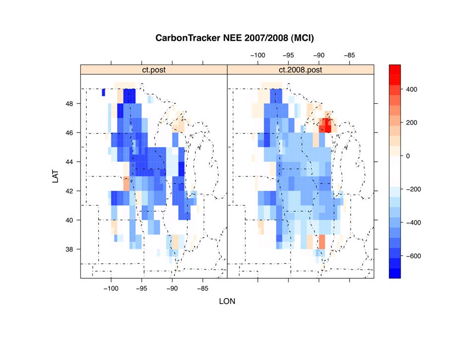
19. Posteriors Priors UMich 2008 CSU 2008 annual nee estimates for 2008 (GgC/gridcell)

20. How do we interpret ? Inversions appear very similar, spatially, in 2007 between CSU and PSU and in 2008 between CSU and Umich However, we see significantly different magnitude of sources/sinks between CSU and the other two, with CSU having an estimated sink much weaker than the MCI inventory How do we diagnose?

21. Transport Uncertainty Summer time sensitivity (to surface) is stronger in CSU than PSU More similar in winter time Could this be why flux corrections are too weak in CSU’s inversion in summer? Poster Andrews E-119

22. Transport Uncertainty Stronger sensitivity in LPDM-RAMS than STILT- WRF for top of LEF tower (afternoon obs) Poster Andrews E-119 … however LPDM- SiBRAMS seem to match observation pretty well

23. Summary on inversions as group In general, NEE from two of the three inversions appear to be in general vicinity of the inventory and the third (CSU) shows similar spatial traits to the others but needs investigation into absolute source/sink strength Mesoscale inversions show promise at inversion grid resolutions generally not possible in most global inversions Continued work is needed to compare the transport fields which currently show significant differences (WRF- STILT, WRF-LPDM and RAMS-LPDM) Would like to continue investigation of differences between inventory and inversion results which have appeared for 2008.