1. Geometric Approaches to Reconstructing Time Series Data Final Presentation 10 May 2007 CSC/Math 870 Computational Discrete Geometry Connie Phong

2. Recap Objective: To reconstruct a time ordering from unordered data This representative dataset is mRNA expression levels in yeast: it has 500 dimensions and includes 18 time points

3. Recap Estimated a time ordering from a MST-diameter path construction (Magwene et al. 2003) A PQ tree represents the uncertainties and defines a permutation subset that contains the true ordering 1 234567 8 917 10 18 16 11 121314 15

4. Recap The MST-diameter path construction is not satisfactory. –The approach is not really rooted in theory –Outputs a large number of possible orderings without providing a means to sort through them Refined objective: To develop a rigorous algorithm/heuristic to reconstruct a temporal ordering from unordered microarray data

5. The Kalman Filter Given: A sequence of noisy measurements Want: To estimate internal states of the process The Kalman filter provides an optimal recursive algorithm that minimizes the mean-square-error. The Kalman filter assumes: –The process can be described by a linear model. –The process and measurement noises are white. –The process and measurement noises are Gaussian. x k = Ax k-1 + Bu k-1 + w k-1 z k = Hx k + v k p(w) ~ N(0, Q) p(v) ~ N(0, R)

6. A Conceptual Explanation Consider the conditional probability density function of x –x(i) conditioned on knowledge of the measurement z(i) = z 1 The assumption that process and measurement noises are Gaussian imply that there’s a unique best estimate of x.

7. Discrete Kalman Filter Algorithm Time-Update: “Predict” Measurement-Update: “Correct” –The Kalman gain term K is chosen such that mean square error of the a posteriori error is minimized Initial estimates

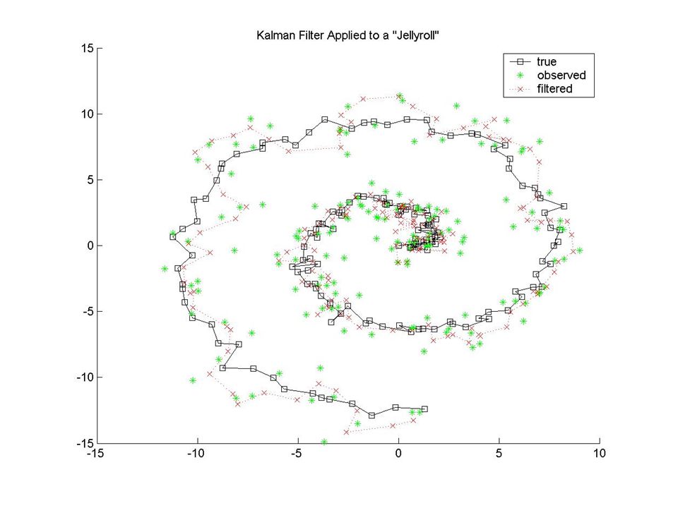
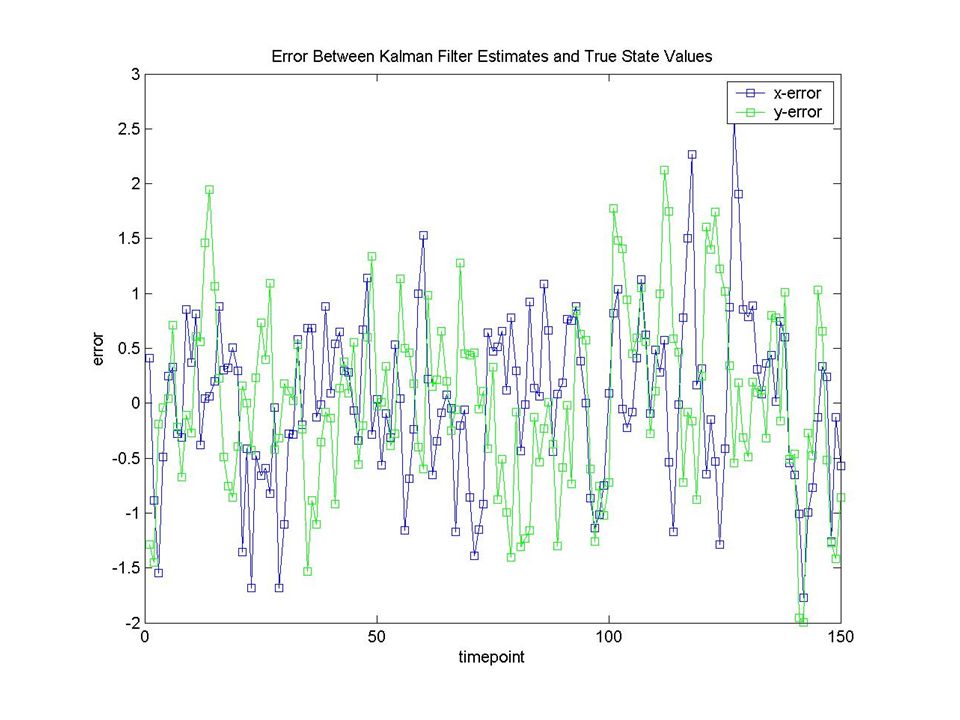
8. Implementing the Kalman Filter Consider a particle with initial position (10, 10) moving with constant velocity 1 m/s through 2D space and trajectory subject to random perturbations The linear model: x k = Ax k-1 + w k-1 z k= Hx k + v k

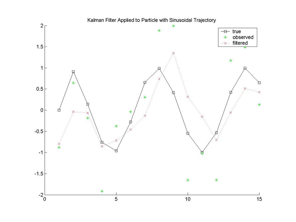
11. Implementing the Kalman Filter Consider a sinusoidal trajectory with linear model: x k = Ax k-1 + w k-1 z k= Hx k + v k

16. Apply the Kalman Filter to Microarray Data General Idea: –Estimate the expression profile x k –Compare x k to raw data to find the best match –The matching data point takes time k The obstacle now is finding a linear model –For example, what should the n x n matrix A be? In the yeast data set n = 500; what are implications of reducing dimensions? Want the simplest way to represent overall induction level and change in induction level over time. –Assumptions of white, Gaussian noise are reasonable

17. Proposed Scheme Start Kalman filter from the most well-defined subsequence of the MST-diameter path estimated ordering Want Kalman filter to “filter” through this partial ordering but “smooth” and/or “predict forward” from its bounds –Compare these estimated past/future states with the actual measurements