Download presentation
Presentation is loading. Please wait.

1
1 Econ 240A Power 7

2
2 Last Week §Normal Distribution §Lab Three: Sampling Distributions §Interval Estimation and HypothesisTesting

3
3 Outline §Distribution of the sample variance §The California Budget: Exploratory Data Analysis §Trend Models §Linear Regression Models §Ordinary Least Squares

4
4 The Sample Variance, s 2 Is distributed with n-1 degrees of freedom (text, 12.3 “inference about a population variance) (text, pp. 258-262, Chi-Squared distribution)
.")
5
5 Text Chi-Squared Distribution

6
6 Text Chi-Squared Table

7
7 Example: Lab Three §50 replications of a sample of size 50 generated by a Uniform random number generator, range zero to one. l expected value of the mean: 0.5 l expected value of the variance: 1/12

8
8 Histogram of 50 Sample Means, Uniform, U(0.5, 1/12) Average of the sample means: 0.4963
 Average of the sample means:")
9
9 Histogram of 50 sample variances, Uniform, U(0.5, 0.0833) Average sample variance: 0.08352
 Average sample variance:")
10
10 Confidence Interval for the first sample variance of 0.07667 §A 95 % confidence interval Where taking the reciprocal reverses the signs of the inequality

11
11

12
12 The UC Budget

13
13 The UC Budget §The part of the UC Budget funded by the state from the general fund

14
14

15
15

16
16 Appendix p. 25

17
17 Appendix p. 25

18
18 Appendix p. 47

19
19

20
20 P. 98

21
21 P. 98

22
22 P. 99

23
23

24
24 How to Forecast the UC Budget? §Linear Trendline?

25
25 Trend Models

26
26

27
27 Forecast increase $84 million

28
28 Linear Regression Trend Models §A good fit over the years of the data sample may not give a good forecast

29
29 How to Forecast the UC Budget? §Linear trendline? §Exponential trendline ?

30
30 Forecast growth rate: 6.8%/yr

31
31 Time Series Models §Linear l UCBUD(t) = a + b*t + e(t) l where the estimate of a is the intercept: $-10.56 million in 68-69 l where the estimate of b is the slope: $84 million/yr l where the estimate of e(t) is the the difference between the UC Budget at time t and the fitted line for that year §Exponential
 = a + b*t + e(t) l where the estimate of a is the intercept: $ million in l where the estimate of b is the slope: $84 million/yr l where the estimate of e(t) is the the difference between the UC Budget at time t and the fitted line for that year §Exponential")
32
32 intercept slope Error in 01-02

33
33 Time Series Models §Exponential l UCBUD(t) = UCBUD(68-69)*e b*t e e(t) l UCBUD(t) = UCBUD(68-69)*e b*t + e(t) l where the estimate of UCBUD(68-69) is the estimated budget for 1968-69 l where the estimate of b is the exponential rate of growth
 = UCBUD(68-69)*e b*t e e(t) l UCBUD(t) = UCBUD(68-69)*e b*t + e(t) l where the estimate of UCBUD(68-69) is the estimated budget for l where the estimate of b is the exponential rate of growth")
34
34 Forecast growth rate: 6.8%/yr 1 year forecast from 2003-04 1.068*3038.666 = 3245.295 M$ Exponential rate of growth Estimated UCBUD in 68-69

35
35 Linear Regression Time Series Models §Linear: UCBUD(t) = a + b*t + e(t) §How do we get a linear form for the exponential model?
 = a + b*t + e(t) §How do we get a linear form for the exponential model")
36
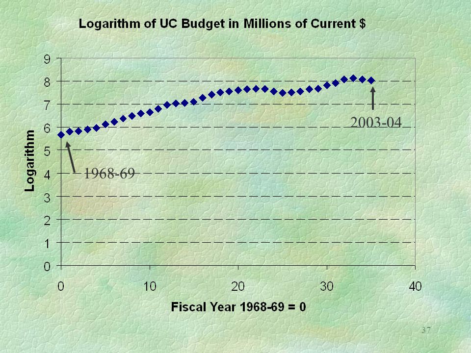
36 Time Series Models §Linear transformation of the exponential l take natural logarithms of both sides l ln[UCBUD(t)] = ln[UCBUD(68-69)*e b*t + e(t) ] l where the logarithm of a product is the sum of logarithms: l ln[UCBUD(t)] = ln[UCBUD(68-69)]+ln[e b*t + e(t) ] l and the logarithm is the inverse function of the exponential: l ln[UCBUD(t)] = ln[UCBUD(68-69)] + b*t + e(t) l so ln[UCBUD(68-69)] is the intercept “a”
![36 Time Series Models §Linear transformation of the exponential l take natural logarithms of both sides l ln[UCBUD(t)] = ln[UCBUD(68-69)*e b*t + e(t) ] l where the logarithm of a product is the sum of logarithms: l ln[UCBUD(t)] = ln[UCBUD(68-69)]+ln[e b*t + e(t) ] l and the logarithm is the inverse function of the exponential: l ln[UCBUD(t)] = ln[UCBUD(68-69)] + b*t + e(t) l so ln[UCBUD(68-69)] is the intercept a](http://images.slideplayer.com/16/5226681/slides/slide_36.jpg "36 Time Series Models §Linear transformation of the exponential l take natural logarithms of both sides l ln[UCBUD(t)] = ln[UCBUD(68-69)*e b*t + e(t) ] l where the logarithm of a product is the sum of logarithms: l ln[UCBUD(t)] = ln[UCBUD(68-69)]+ln[e b*t + e(t) ] l and the logarithm is the inverse function of the exponential: l ln[UCBUD(t)] = ln[UCBUD(68-69)] + b*t + e(t) l so ln[UCBUD(68-69)] is the intercept a")
37
37 1968-69 2003-04
38
38 Exponential rate of growth ln UCBUD at t=0 exp[5.932] = 376.9 observed = $291.3
![38 Exponential rate of growth ln UCBUD at t=0 exp[5.932] = observed = $291.3](http://images.slideplayer.com/16/5226681/slides/slide_38.jpg "38 Exponential rate of growth ln UCBUD at t=0 exp[5.932] = observed = $291.3")
39
39 Forecast growth rate: 6.8%/yr Exponential rate of growth Estimated UCBUD in 68-69

40
40 Naïve Forecasts §Average §forecast next year to be the same as this year

41
41

42
42 UC Budget Forecasts for 2004-05 * 1.068x$3,038,666,000; exponential trendline forecast ~$4.3 B

43
43 Time Series Forecasts §The best forecast may not be a regression forecast §Time Series Concept: time series(t) = trend + cycle + seasonal + noise(random or error) §fitting just the trend ignores the cycle §UCBUD(t) = a + b*t + e(t)
 = trend + cycle + seasonal + noise(random or error) §fitting just the trend ignores the cycle §UCBUD(t) = a + b*t + e(t)")
44
44 Ordinary Least Squares

45
45 intercept slope Error in 01-02

46
46 Criterion for Fitting a Line §Minimize the sum of the absolute value of the errors? §Minimize the sum of the square of the errors l easier to use §error is the difference between the observed value and the fitted value l example UCBUD(observed) - UCBUD(fitted)
 - UCBUD(fitted).")
47
47 §The fitted value: §The fitted value is defined in terms of two parameters, a and b (with hats), that are determined from the data observations, such as to minimize the sum of squared errors
, that are determined from the data observations, such as to minimize the sum of squared errors")
48
48 Minimize the Sum of Squared Errors

49
49 How to Find a-hat and b-hat? §Methodology l grid search l differential calculus l likelihood function

50
50 Grid Search, a-hat=0, b-hat=80

51
51 Grid Search a-hat - + + - 0 b-hat Find the point where the sum of squared errors is minimum

52
52 Differential Calculus §Take the derivative of the sum of squared errors with respect to a-hat and with respect to b-hat and set to zero. §Divide by -2*n §or

53
53 Least Squares Fitted Parameters §So, the regression line goes through the sample means. §Take the other derivative: §divide by -2

54
54 Ordinary Least Squares(OLS) §Two linear equations in two unknowns, solve for b-hat and a-hat.
 §Two linear equations in two unknowns, solve for b-hat and a-hat.")
55
55 Dependent Variable: UCBUD Method: Least Squares Dependent Variable: UCBUD Sample: 1968 2003 Included observations: 36 VariableCoefficientStd. Errort-StatisticProb. C73.4401476.450540.9606230.3435 T84.003883.75658322.361780.0000 R-squared0.936335 Mean dependent var1543.5 Adjusted R-squared0.934463 S.D. dependent var914.62 S.E. of regression 234.1469 Akaike info criterion13.803 Sum squared resid1864043. Schwarz criterion13.891 Log likelihood-246.4671 F-statistic 500.04 Durbin-Watson stat0.339456 Prob(F-statistic)0.000000
")
56
56

Similar presentations


 White noise input output Random walkSynthesis 1/(1 – bz) White noise input output.>")


