1. Contents Distributed Sensor Networks (DSNs) Key Predistribution Schemes – KPSs A Set System The 3 phases Metrics for the Evaluation of KPSs Configurations Linear schemes Quadratic schemes Performance comparisons

2. Contents Distributed Sensor Networks (DSNs) Key Predistribution Schemes – KPSs A Set System The 3 phases Metrics for the Evaluation of KPSs Configurations Linear schemes Quadratic schemes Performance comparisons

3. Introduction Distributed sensor networks (DSNs) –What are they?

4. Introduction Distributed sensor networks (DSNs) –What are they? –What for? Civilian areas –Forest fire sensors –Sensors of vibrations to predict earthquakes –Sensors of chemical substances to discover pollution

6. Introduction Distributed sensor networks (DSNs) –What are they? –What for? Civilian areas –Forest fire sensors –Sensors of vibrations to predict earthquakes –Sensors of chemical substances to discover pollution Military applications –Collecting images –Collecting sounds

7. Requirements Accumulate secret information (and relay it to a base station) Communicate with each other As small as possible Consume little power Encryption

8. Encryption is the process of transforming information (referred to as plaintext) using an algorithm (called cipher) to make it unreadable to anyone except those possessing special knowledge, usually referred to as a key.

9. Two trivial examples Every node is given the same secret “master key” Low Memory costs Compromise of a single node would render the network completely insecure and unreliable For every pair of nodes and there is a secret key given only to these 2 nodes Expensive memory costs Excellent resiliency (security)

10. Ways to establish pairwise secret keys Using public key protocols Expensive computational costs Increased storage requirements Establishing a trusted server that can communicate with all the nodes in the network (like Kerberos) Expensive costs for message relay Employing key predistribution schemes (also called KPSs)

11. Contents Distributed Sensor Networks (DSNs) Key Predistribution Schemes – KPSs A Set System The 3 phases Metrics for the Evaluation of KPSs Configurations Linear schemes Quadratic schemes Performance comparisons

12. Related Prior Work Several schemes were proposed for KPS The schemes we will be discussing closely rely on previous work We will mention 7 other schemes

13. The Basic Scheme Developed by Eschenauer and Gligor 3 Parameters: –n number of nodes –k size of key ring –v size of key space Nodes communicate if they have a shared key –Encryption is done using the shared key

14. The Basic Scheme n can grow greatly even for medium values of v and k

15. Basic scheme: Deterministic vs Randomized Key Rings Randomized Keys are chosen by random Key ring assignment is done by random Deterministic Keys are still chosen by random! Key ring assignment is deterministic

16. Basic scheme: Deterministic vs Randomized Key Rings Deterministic No overhead Combinatorial properties are guaranteed. Shared-key discovery and path key establishments can be done in O(1). Randomized Significant overhead in generating good pasudo- random numbers Combinatorial properties are not guaranteed (such as connectivity) Shared-key discovery and path key establishments – O(???)

17. q Composite Scheme Generalization of the Basic Scheme Two nodes communicate directly if they have at least q common keys –Encryption key is created using all common keys If q=1 then similar to Basic Scheme, yet different

18. Camtepe and Yener’s Scheme First scheme to use combinatorial designs called Set Systems Blocks and points

19. 2005 Lee and Stinson’s Scheme Authors of the article Set Systems Linear polynomials over a finite field

20. Chakrabarti, Maitra, and Roy’s Scheme Start with a certain Set System Form key rings by merging blocks Larger key rings Some performance metrics are improved

21. Multiple Space Schemes Combine basic KPS (set systems) with older KPS such as Blom[1985] Inner and outer schemes

22. Multiple Space Schemes Blom [1985]

23. Hash Chain Schemes Another avenue of research using KPS Good resilience Bad complexity

24. Contents Distributed Sensor Networks (DSNs) Key Predistribution Schemes – KPSs A Set System The 3 phases Metrics for the Evaluation of KPSs Configurations Linear schemes Quadratic schemes Performance comparisons

25. A Set System A set system is a pair (X,A) A is a finite set of subsets of X called blocks The degree of a point is the number of blocks containing x )X,A) is regular if (of degree r) if all points have the same degree r The rank of (X,A) is the size of the largest block. If all blocks have the same size, say k, then (X,A) is said to be uniform (of rank k)

26. Example X={1,2,3,4,5,6,7,8,9} A={123,456,789,147,258,369 159,267,348,168,249,357}

27. Contents Distributed Sensor Networks (DSNs) Key Predistribution Schemes – KPSs A Set System The 3 phases Metrics for the Evaluation of KPSs Configurations Linear schemes Quadratic schemes Performance comparisons

28. The 3 phases –There are 3 basic operation that should be implemented: Key predistribution Shared-key discovery Path-key establishment

29. Key Predistribution Phase Choose n and k input parameters Center creates a uniform and regular set system with rank k and n blocks Center determines q Assignment algorithm What happens if A is just a set of n random k sized blocks?

30. Shared-Key Discovery phase The phase in which 2 nodes determine the common points in the 2 blocks assigned to them –Suggestion: node i would broadcast the k points in to each of its neighbors Suppose that 2 nodes discover that and have exactly t common points : if t>=q then they can establish a secret key

31. The secret key h is a public key derivation function (such as SHA-1) We are using all the common keys to derive the pairwise key in order to achieve maximum resiliency!

32. Path-Key Establishment phase What happens if 2 nodes in wireless communication rage fail to find sufficient number of common keys in the shared-key discovery phase? –They look for multiple secure links (or hops) to reach each other

33. Contents Distributed Sensor Networks (DSNs) Key Predistribution Schemes – KPSs A Set System The 3 phases Metrics for the Evaluation of KPSs Configurations Linear schemes Quadratic schemes Performance comparisons

34. Metrics for the Evaluation of KPSs Network Size (denoted by n) Key Storage (denoted by k) Global connectivity Local connectivity Resiliency Complexity of Shared-Key Discovery and Path-Key Establishment

35. Network Size The number of nodes in a DSN, which we denote by the parameter n. –The number of nodes is usually between 1,000 and 10,000 nodes (or even higher) –Notice that in some schemes cannot be chosen independently!

36. Key Storage The number of keys per node, which we denote by the parameter k –When we use a combinatorial set system as a key ring space, the number of keys per node is equal to the rank of the set system, which is denoted by k

37. Global Connectivity The communication capabilities of the network –It is depended on the physical level and the network level The Physical Level is represented by the physical graph The Network Level is represented by the block graph –Determined by the structure of the key ring space

38. They Key-Sharing Graph It is the intersection between the physical graph and the block graph We hope that the key sharing graph is connected We say that the DSN is globally connected if the key sharing graph is a connected graph

39. Local Connectivity Refers to the situation where nodes that are physically close to each other can establish a short secure communication path between them Pr1 – The probability that 2 random nodes share at least q common keys Pr2 – The probability that 2 nodes in wireless communication range do not share q common keys but there exist a third node that shares q common keys with each of the first 2 nodes

40. Resiliency When an adversary captures a number of sensor nodes at random we assume that all the keys of information stored in the nodes are revealed to the adversary. We want node captures to affect as small a part of the entire network as possible The resiliency of the network is estimated by fail(s), which is the probability that a link between 2 fixed noncompromised nodes is affected after s other nodes are compromised

41. Complexity of Shared-Key Discovery and Path-Key Establishment Shared-Key discovery is often done by having the 2 nodes exchange the list of identifiers of the keys they hold If the 2 lists are presorted in increasing order of key identifiers then this can be done in time O(k) By choosing carefully structured key ring space we can obtain an algebraic description of the key rings In that case we can reduce the computational complexity of shared-key discovery to O(1)!!!

42. Contents Distributed Sensor Networks (DSNs) Key Predistribution Schemes – KPSs A Set System The 3 phases Metrics for the Evaluation of KPSs Configurations Linear schemes Quadratic schemes Performance comparisons

43. Configurations We’ll have q=1 for the rest of the discussion (v,n,r,k)-designs Necessary condition for existing configuration nk = vr

44. LEMMA 1 Any vertex (i.e., block) A j in the block graph GA of a (v, n, r, k)-design, (X,A), has degree at most k(r − 1). Further, all vertices in GA have degrees equal to k(r−1) if and only if |Ai ∩ A j| ≤ 1 for all

45. Configurations A (v, n, r, k)-design is called a (v, n, r, k)- configuration if any two distinct blocks intersect in zero or one point.

46. LEMMA 2 Suppose we use a (v, n, r, k)-design for a key ring space with intersection threshold q = 1. Then Pr1 ≤ k(r − 1)/(n − 1). Further, Pr1 = k(r− 1)/(n− 1) if and only if the (v, n, r, k)-design is a configuration.

47. LEMMA 3 A (v, n, r, k)-configuration exists only if nk = vr and v − 1 ≥ r(k − 1).

48. Complete Block Graphs The block graph of a configuration is a complete graph if and only if k(r − 1) = n − 1 n << k²

49. μ-Common Intersection Designs Two-hop paths Increase choices for best-match common neighbor

50. μ-Common Intersection Designs Suppose that (X,A) is a (v, n, r, k)- configuration. We say that (X,A) is a μ-common intersection design (or (v, n, r, k;μ)-CID) provided that whenever Ai ∩ A j = ∅.

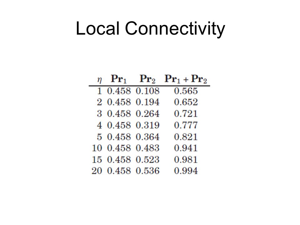
51. Pr1 and Pr2 η - number of nodes in the intersection of the neighborhoods of the two nodes Ui and Uj.

52. Contents Distributed Sensor Networks (DSNs) Key Predistribution Schemes – KPSs A Set System The 3 phases Metrics for the Evaluation of KPSs Configurations Linear schemes Quadratic schemes Performance comparisons

53. Linear Schemes A Tranversal design TD(k,m) is a Triple (X,H,A) X is a finite set of cardinality km H is a partition of X into k parts of size m A is a set of k-subsets of X called blocks * ** Every pair x,y from different groups occurs in exactly one block in A

54. Theorem If there exists a TD(k,m) then there is a (km, m*m,m,k;k*k-k)-CID Proof: it is not hard to see that a TD(k,m) has km points and m*m blocks, every block has size k, and every point ocuurs in m blocks

55. Proof cont’ Next, we show that (X,A) is a configuration Let A1, A2 be two blocks and suppose that Therefore there are 2 points x1, x2 such that from * x1 and x2 must be from different groups. from ** we get a contradiction

56. Proof cont’ Finally we show that (X,A) is a CID Suppose and where A and B are 2 disjoint blocks There is no block containing the pair but there is unique block containing any pair where Hence, the design is a common intersection design

57. LEMMA It is well-known (from previous articles) that if p is a prime or prime power, the TD(k,p) can be easily constructed.

58. Example

59. TD(30, 49) key ring space (1470, 2401, 49, 30)-1-design support up to 2,401 nodes in the network every node is required to store 30 keys

60. Local connectivity Pr1 and Pr2:

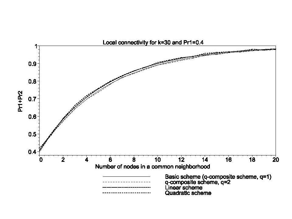
61. Local Connectivity

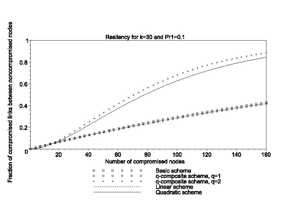
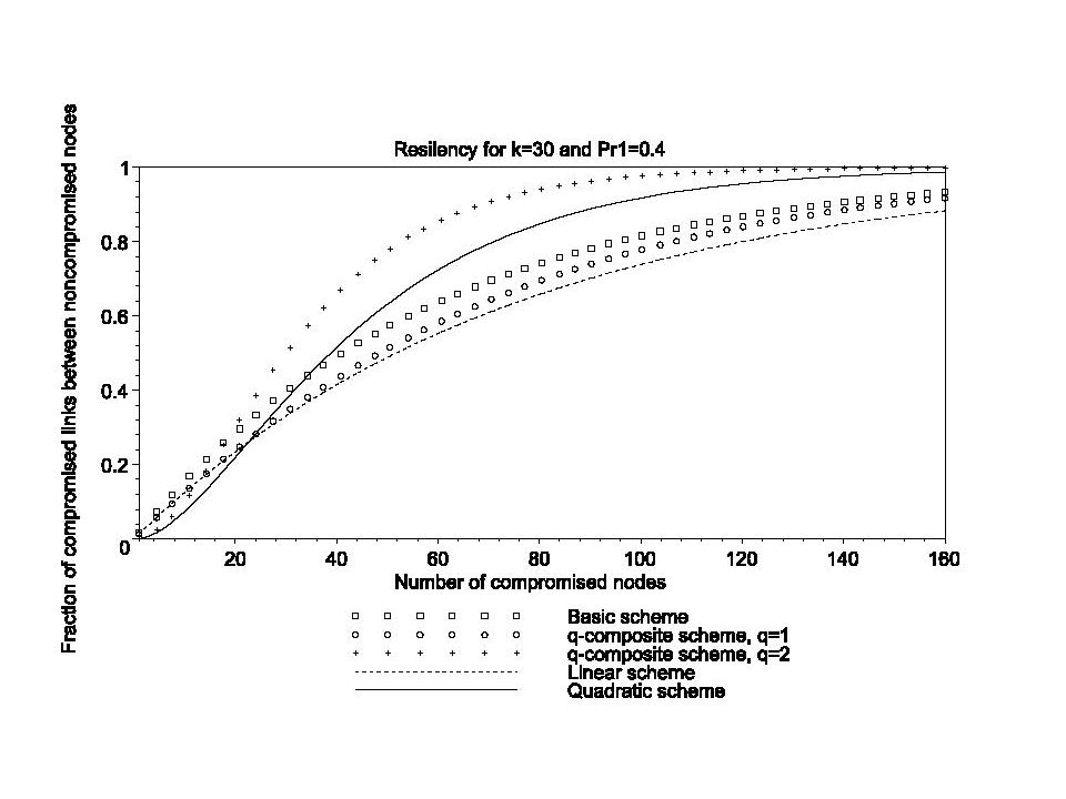
62. Resiliency

63. Network Size

64. Contents Distributed Sensor Networks (DSNs) Key Predistribution Schemes – KPSs A Set System The 3 phases Metrics for the Evaluation of KPSs Configurations Linear schemes Quadratic schemes Performance comparisons

65. Quadratic Schemes A Tranversal design TD(t,k,m) is a Triple (X,H,A) X is a finite set of cardinality km H is a partition of X into k parts of size m A is a set of k-subsets of X called blocks * ** Every subset of t elements of X from t different groups occurs in exactly one block in A A TD(k,m) is identical to a TD(2,k,m)

66. Theorem Suppose (X,H,A) is a TD(3,k,m) Then every point occurs in exactly blocks, and every pair of points from different groups occurs in exactly m blocks. Further, any block intersects exactly blocks in one point, exactly blocks in two points, and is disjoint from exactly blocks

67. proof Let x,y be any 2 points from different groups. Let H be a group such that. Then for every, there is a unique block containing x,y, and z. Hence, there are m blocks containing x, y and some (because the size of H is m). Next, let x be any point and let H be any group such that. For every, there are m blocks containing x and z. The resulting blocks are distinct and account for all the blocks containing x (this follows from **). Now, let A be a block. There are ways to choose 2 points. For each such choice, there are m-1 blocks other than A that contain x and y.

68. Proof cont’ The resulting blocks are distinct and account for all the blocks that intersect A in exactly 2 points. Suppose there are blocks that intersect A in exactly i points, i=0,1,2. We have shown above that Now, suppose that. There are (m-1)(k-1) blocks that contain x and exactly one other point from A. There blocks intersect A in exactly 2 points. There remain blocks other than A that contain x. Since there are k points, it follows that. Finally, since the total number of blocks is, it follows that.

69. Example TD(3, 23, 23) each node in the network is required to store 23 keys

70. Local Connectivity

72. Resiliency

73. Network Size

74. Contents Distributed Sensor Networks (DSNs) Key Predistribution Schemes – KPSs A Set System The 3 phases Metrics for the Evaluation of KPSs Configurations Linear schemes Quadratic schemes Performance comparisons

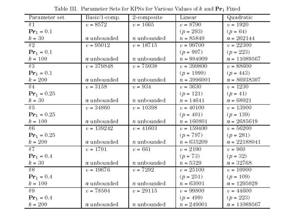
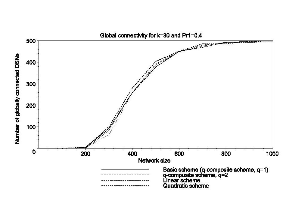
75. Performance Comparisons We will compare the following schemes for different parameter situations: –Basic schmes –1-composite and 2-composite schemes –Linear schemes –Quadratic schemes

83. Summarize All the schemes are able to support quite large networks. The basic, 1-composite and linear schemes require quite large key pools when k is large and Pr1 is small. The linear scheme has the simplest shared-key discovery. As Pr1 decrease the nodes must be distributed more densely in order to have good local connectivity. The quadratic and 2-composite schemes have the best resiliency when k and Pr1 are both large. There is a trade-off between connectivity and resiliency. In general, a larger value of k is beneficial for all the metrics considered.