1. State Estimation and Kalman Filtering CS B659 Spring 2013 Kris Hauser

2. Motivation Observing a stream of data Monitoring (of people, computer systems, etc) Surveillance, tracking Finance & economics Science Questions: Modeling & forecasting Handling partial and noisy observations

3. Markov Chains Sequence of probabilistic state variables X 0,X 1,X 2,… E.g., robot’s position, target’s position and velocity, … X0X0 X1X1 X2X2 X3X3 Observe X 1 X 0 independent of X 2, X 3, … P(X t |X t-1 ) known as transition model

5. Inference in MC Prediction: the probability of future state? P(X t ) =  x0,…,xt-1 P (X 0,…,X t ) =  x0,…,xt-1 P (X 0 )  x1,…,xt P(X i |X i-1 ) =  xt-1 P(X t |X t-1 ) P(X t-1 ) “Blurs” over time, and approaches stationary distribution as t grows Limited prediction power Rate of blurring known as mixing time [Incremental approach]

6. Modeling Partial Observability Hidden Markov Model (HMM) X0X0 X1X1 X2X2 X3X3 O1O1 O2O2 O3O3 Hidden state variables Observed variables P(O t |X t ) called the observation model (or sensor model)

7. Filtering Name comes from signal processing Goal: Compute the probability distribution over current state given observations up to this point X0X0 X1X1 X2X2 O1O1 O2O2 Query variable Known Distribution given Unknown

8. Filtering Name comes from signal processing Goal: Compute the probability distribution over current state given observations up to this point P(X t |o 1:t ) =  x t-1 P(x t-1 |o 1:t-1 ) P(X t |x t-1,o t ) P(X t |X t-1,o t ) = P(o t |X t-1,X t )P(X t |X t-1 )/P(o t |X t-1 ) =  P(o t |X t )P(X t |X t-1 ) X0X0 X1X1 X2X2 O1O1 O2O2 Query variable Known Distribution given Unknown

9. Kalman Filtering In a nutshell Efficient probabilistic filtering in continuous state spaces Linear Gaussian transition and observation models Ubiquitous for state tracking with noisy sensors, e.g. radar, GPS, cameras

10. Hidden Markov Model for Robot Localization Use observations + transition dynamics to get a better idea of where the robot is at time t X0X0 X1X1 X2X2 X3X3 z1z1 z2z2 z3z3 Hidden state variables Observed variables Predict – observe – predict – observe…

11. Hidden Markov Model for Robot Localization Use observations + transition dynamics to get a better idea of where the robot is at time t Maintain a belief state b t over time b t (x) = P(X t =x|z 1:t ) X0X0 X1X1 X2X2 X3X3 z1z1 z2z2 z3z3 Hidden state variables Observed variables Predict – observe – predict – observe…

12. Bayesian Filtering with Belief States

13. Update via the observation z t Predict P(X t |z 1:t-1 ) using dynamics alone Bayesian Filtering with Belief States

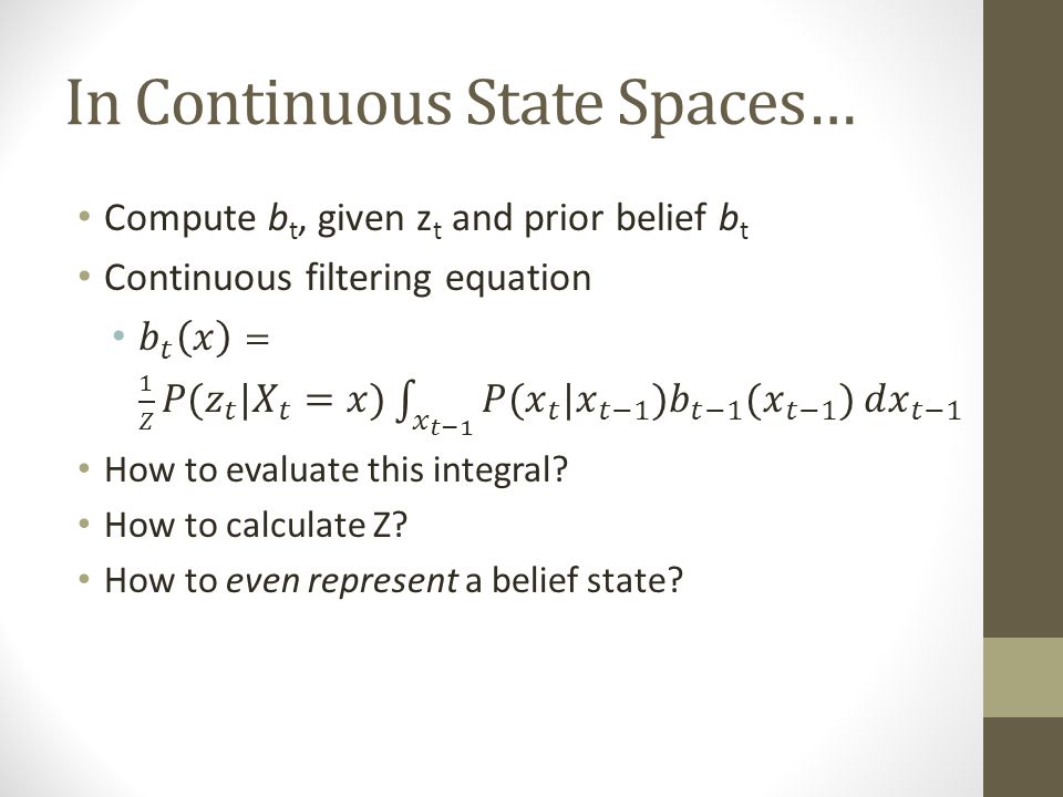
14. In Continuous State Spaces…

16. Key Representational Decisions Pick a method for representing distributions Discrete: tables Continuous: fixed parameterized classes vs. particle-based techniques Devise methods to perform key calculations (marginalization, conditioning) on the representation Exact or approximate?

17. Gaussian Distribution

18. Linear Gaussian Transition Model for Moving 1D Point Consider position and velocity x t, v t Time step h Without noise x t+1 = x t + h v t v t+1 = v t With Gaussian noise of std   P(x t+1 |x t )  exp(-(x t+1 – (x t + h v t )) 2 /(2   2  i.e. X t+1 ~ N(x t + h v t,   )

19. Linear Gaussian Transition Model If prior on position is Gaussian, then the posterior is also Gaussian vh 11 N( ,  )  N(  +vh,  +  1 )

20. Linear Gaussian Observation Model Position observation z t Gaussian noise of std  2 z t ~ N(x t,   )

21. Linear Gaussian Observation Model If prior on position is Gaussian, then the posterior is also Gaussian   (  2 z+  2 2  )/(  2 +  2 2 )  2   2  2 2 /(  2 +  2 2 ) Position prior Posterior probability Observation probability

22. Multivariate Gaussians X ~ N( ,  )

23. Multivariate Linear Gaussian Process A linear transformation + multivariate Gaussian noise If prior state distribution is Gaussian, then posterior state distribution is Gaussian If we observe one component of a Gaussian, then its posterior is also Gaussian y = A x +  ~ N( ,  )

24. Multivariate Computations Linear transformations of gaussians If x ~ N( ,  ), y = A x + b Then y ~ N(A  +b, A  A T ) Consequence If x ~ N(  x,  x ), y ~ N(  y,  y ), z=x+y Then z ~ N(  x +  y,  x +  y ) Conditional of gaussian If [x 1,x 2 ] ~ N([  1  2 ],[  11,  12 ;  21,  22 ]) Then on observing x 2 =z, we have x 1 ~ N(  1 -  12  22 -1 (z-  2 ),  11 -  12  22 -1  21 )

25. Presentation

26. Next time Principles Ch. 9 Rekleitis (2004)