1. EC 723 Satellite Communication Systems
Mohamed Khedr

2. Syllabus Tentatively Week 1 Overview Week 2
Orbits and constellations: GEO, MEO and LEO
Week 3
Satellite space segment, Propagation and satellite links , channel modelling
Week 4
Satellite Communications Techniques
Week 5
Satellite Communications Techniques II
Week 6
Satellite error correction Techniques
Week 7
Multiple Access I
Week 8
Multiple access II
Week 9
Satellite in networks I, INTELSAT systems , VSAT networks, GPS
Week 10
GEO, MEO and LEO mobile communications
INMARSAT systems, Iridium , Globalstar, Odyssey
Week 11
Presentations
Week 12
Week 13
Week 14
Week 15
Tentatively

3. Agenda Modulation Concept Analog Communication Digital Communication
Digital Modulation Schemes

4. EFFECT OF FILTERING - 1
Fig. 5.8 in text

5. EFFECT OF FILTERING - 2
Rectangular pulses (i.e. infinite rise and fall times of the pulse edges) need an infinite bandwidth to retain the rectangular shape
Communications systems are always band-limited, so
send a SHAPED PULSE
Attempt to MATCH the filter to the spectrum of the energy transmitted
Before FILTERS, let’s look at Inter-Symbol Interference

6. INTER-SYMBOL INTERFERENCE
Sending pulses through a band-limited channel causes “smearing” of the pulse in time
“Smearing” causes the tail of one pulse to extend into the next (later) pulse period
Parts of two pulses existing in the same pulse period causes Inter-Symbol Interference (ISI)
ISI reduces the amplitude of the wanted pulse and reduces noise immunity
Example of ISI

7. ISI - contd. - 1
Form Couch, Fig. 3-23

8. ISI - contd. - 2
To avoid ISI, you can SHAPE the pulse so that there is zero energy in adjacent pulses
Use NRZ; pulse lasts the full bit period
Use Polar Signaling (+V & -V); average value is zero if equal number of 1’s and 0’s
Communications links are usually AC coupled so you should avoid a DC voltage component
Then use a NYQUIST filter
Nyquist Filter???

9. NYQUIST FILTER - 1 Bit Period is Tb
Sampling of the signal is usually at intervals of Tb
Thus, if we could generate pulses that are at a one-time maximum at t = Tb and zero at each succeeding interval of Tb (i.e. t = 2Tb, 3Tb, ….. , NTb then we would have no ISI
This is called a NYQUIST filter

10. Sampling instant is CRITICAL
NYQUIST FILTER - 2
Sampling instant is CRITICAL
Impulse at this point t
Tb Tb Tb Tb

11. NYQUIST FILTER - 3
NOTE: At each sampling interval, there is only one pulse contribution - the others being at zero level
Fig. 5.9 in text

12. NYQUIST FILTER - 4
Arranging to sample at EXACTLY the right instant is the “Zero ISI” technique, first proposed by Nyquist in 1928
Networks which produce the required time waveforms are called “Nyquist Filters”. None exist in practice, but you can get reasonably close

13. NYQUIST FILTER - 5 Noise into receiver must be held to a minimum
Place half of Nyquist filter at transmit end of link, half at receive end, so that the individual filter transfer function H(f) is given by Vr(f)NYQUIST = H(f)  H(f) Filter is a “Square Root Raised Cosine Filter”
H(f) matches pulse characteristic, hence it is called a “matched filter”
Matched Filter

14. MATCHED FILTER - 1 Roll-off factor =  = (f / f0 )
where f0 = 6 dB bandwidth
B = absolute bandwidth (here shown for  = 0.5) and
B = f f0
f1 = start of ‘roll-off’ of the filter characteristic
6 dB f1 f0 B

15. BUT how much bandwidth is required for a given transmission rate???
MATCHED FILTER - 2
A Raised Cosine Filter gives a Matched Filter response
The “Roll-Off Factor”, , determines bandwidth of Raised Cosine Low Pass Filter (LPF)
Gives zero ISI when the output is sampled at correct time, with sampling rate of Rb (i.e. at a sampling interval of Tb)
BUT how much bandwidth is required for a given transmission rate???

16. NOTE: It is the Symbol Rate that is key to bandwidth, not the Bit Rate
BANDWIDTH REQUIRED - 1
Bandwidth required depends on whether the signal is at BASEBAND or at PASSBAND
Bandwidth needed to send baseband digital signal using a Nyquist LPF is Bandwidth = (1/2)Rb(1 + )
Bandwidth needed to send passband digital signal using a Nyquist Bandpass filter is bandwidth = Rb(1 + )
NOTE: It is the Symbol Rate that is key to bandwidth, not the Bit Rate

17. BANDWIDTH REQUIRED - 2
SYMBOL RATE is the number of digital symbols sent per second
BIT RATE is the number of digital bits sent per second
Different modulation schemes will “pack” different numbers of Bits in a single Symbol
BPSK has 1 bit per symbol
QPSK has 2 bits per symbol

18. BANDWIDTH REQUIRED - 3
OCCUPIED BANDWIDTH, B, for a signal is given by B = Rs ( 1 +  ) where Rs is the symbol rate and  is the filter roll-off factor
NOISE BANDWIDTH, BN, for a channel will not be affected by the roll-off factor of filter. Thus BN = Rs

19. BANDWIDTH EXAMPLE - 1 GIVEN:
Bit rate 512 kbit/s
QPSK modulation
Filter roll-off, , is  = 0.3
FIND: Occupied Bandwidth, B, and Noise Bandwidth, BN
SOLUTION: Symbol Rate = Rs = (1/2)  (512  103) = 256  103
2 bits per symbol
Number of bits/s

20. BANDWIDTH EXAMPLE - 2
Occupied Bandwidth, B, is B = Rs (1 +  ) = 256  103 ( ) = kHz
Noise Bandwidth, BN, is BN = Rs = 256 kHz
Now what happens if you have FEC?
Example with FEC

21. BANDWIDTH EXAMPLE - 3 SAME Example, but 1/2-rate FEC is now used
SOLUTION Symbol Rate, Rs = (1/2)  (2)  (512  103) = 512  103 symbols/s Occupied Bandwidth, B, is B = Rs ( 1 +  ) = kHz
2 bits per symbol
1/2-rate FEC used
Number of bits/s

22. BANDWIDTH EXAMPLE - 3
Noise Bandwidth, BN, is BN = Rs = 512  103 = 512 kHz
Summary:
High Modulation Index  More Bandwidth Efficient
FEC (Block or Convolutional)  Increases bandwidth required

23. Digital Modulations
Functional model of passband data transmission system

24. Digital Modulations
In digital communications, the modulating signal is a binary or M-ary data.
The carrier is usually a sinusoidal wave.
Change in Amplitude: Amplitude-Shift-Keying (ASK)
Change in Frequency: Frequency-Shift-Keying (FSK)
Change in Phase: Phase-Shift-Keying (PSK)
Hybrid changes (more than one parameter).
Ex. Phase and Amplitude change: Quadrature Amplitude Modulation (QAM)

25. Binary Modulations – Basic Types
These two have constant envelope (important for amplitude sensitive channels)

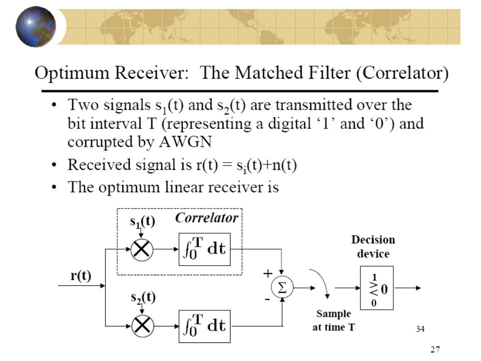
26. Coherent and Non-coherent Detection
Coherent Detection (most PSK, some FSK):
Exact replicas of the possible arriving signals are available at the receiver.
This means knowledge of the phase reference (phased-locked).
Detection by cross-correlating the received signal with each one of the replicas, and then making a decision based on comparisons with pre-selected thresholds.
Non-coherent Detection (some FSK, DPSK):
Knowledge of the carrier’s wave phase not required.
Less complexity.
Inferior error performance.

28. Design Trade-offs Primary resources: Design goals: Transmitted Power.
Channel Bandwidth.
Design goals:
Maximum data rate.
Minimum probability of symbol error.
Minimum transmitted power.
Minimum channel bandiwdth.
Maximum resistance to interfering signals.
Minimum circuit complexity.

29. Coherent Binary PSK (BPSK)
Two signals, one representing 0, the other 1.
Each of the two signals represents a single bit of information.
Each signal persists for a single bit period (T) and then may be replaced by either state.
Signal energy (ES) = Bit Energy (Eb), given by:
Therefore 

30. Orthonormal basis representation
Gram-Schmidt Orthogonalization: basis of signals that are both ortogornal between them and normalized to have unit energy.
Allows representation of M energy signals {si(t)} as linear combinations of N orthonormal basis functions, where N<=M.
Ex.: N=2

31. BPSK representation
Let’s consider the unidimensional base (N=1) where:
Let’s also rewrite the signal amplitudes as a function of their energy:

32. BPSK representation
Therefore, we can write the signals s1(t) and s2(t) in terms of 1(t):
Which can be graphically represented as:

33. BPSK Physical Implementation

34. Detection of BPSK Actual BPSK signal is received with noise
We assume AWGN in this class
Other noise properties are possible
AWGN is a good approximation
Other noise models are more complex
Constellation becomes a distribution because of noise variations to signal

35. Recall Gaussian Distribution
Area to the right of this line represents Probability (x>x0)
= mean
=standard deviation  x0 x
Approximation for large positive values of y 
Where:
Both Q(.) and erfc(.) functions are integrals widely tabled and available as functions in Excel and calculators

36. Calculating Error Probability
Noise Spectral Density = N0
Noise Variance:
BPSK error probability

37. Bit Error Rate (BER) for BPSK
BER is therefore given by
Approximation
valid for Eb/No
greater than ~4 dB
Eb/No
(dB) BER
0 0.08
2 0.04
8 2*10-4
10 4*10-6
Note that these calculations are for synchronous detection

38. Ambiguity Resolution
We haven’t discussed yet how to tell which signal state is a 1 and which a 0
Because of variations in the signal path, its impossible to tell a priori
Two common approaches resolutions:
Unique Word
Differential Encoding

39. Unique Word Ambiguity Resolution
A specific, known unique word is sent
The unique word is sent at a known time in the data
The correct signal state is chosen as 1 to correctly decode the unique word
Usually implemented with two detectors - the output of the correct one is simply used
Could lead to problems until a new UW is RX if a phase slip occurs
All bits after slip will be received wrong!

40. Differential Encoding Ambiguity Resolution
Data is not transmitted directly
Each bit is represented by:
0 => phase shift of p radians
1 => no phase shift
in the carrier
This results in ~ doubling the BER since any error will tend to corrupt 2 bits
BER is then
Valid for BER<~0.01

41. Coherent Quaternary PSK (QPSK)
Four signals are used to convey information
This leads to a constellation of: when shown as a phasor referenced to the signal phase, q
Each of the two states represents a two bits of information
Constant Modulus =>

42. QPSK Constellation Representation
In this case we use the following orthonormal basis:
Which gives, after application of some trigonometric identities, the following constellation representation:

43. QPSK Constellation

44. QPSK Waveform

45. QPSK Physical Implementation
Note that the QPSK
signal can be seen to
be two BPSK signals
in phase quadrature

46. Block diagrams of (a) QPSK transmitter and (b) coherent QPSK receiver.

47. The two QPSK constellations. Note that they differ by п /4
The two QPSK constellations. Note that they differ by п /4. When going from (1,1) to (-1, -1), the phase is shifted by п. When going from (1, -1) to (1,1), the phase shifts by п /2. Thus, depending on the incoming symbol, transitions from (1,1) can occur to (1,1), (1,-1), (-1, 1), or (-1, -1) or vice versa, leading to phase shifts of 0, ± п /2, or ± п in QPSK. I and Q represent the in-phase and quadrature bits, respectively. Arrows show all possible transitions.

48. Bit Error Rate (BER) for QPSK
The BER is still the probability of choosing the wrong signal state (symbol now)
Because the signal is Gray coded (00 is next to 01 and 10 for instance but not 11) the BER for QPSK is that for BPSK:
BER (after a lot of derivation) is given by:
Approximation
valid for Eb/No
greater than ~4 dB
Note that Eb is here, not Es!

49. Possible paths for switching between the message points in (a) QPSK and (b) offset QPSK.

50. Block diagram of the OQPSK modulator.

51. Explanation of the phase transitions in OQPSK.

52. Two commonly used signal constellations of QPSK; the arrows indicate the paths along which the QPSK modulator can change its state.

53. Eight possible phase states for the p/4-shifted QPSK modulator.

54. Phase encoding for  /4-QPSK
Phase encoding for  /4-QPSK. The brackets [ ] and { } correspond to the two respective constellations.

55. Details of the phase constellation associated with п/4-QPSK
Details of the phase constellation associated with п/4-QPSK. For every alternate symbol, the carrier waves are changed. From (1,1) to (-1, -1), we go from [1 1] to {-1, -1}, or from {1,1} to [-1, -1], resulting in a phase change of п /4, as opposed to п/2 in QPSK. In QPSK we can go from [1, 1] to [-1, -1] or from {1 1} to {-1, -1}, resulting in a phase change of п. Also, when we go from (1, 1) to (1, 1) in п/4-QPSK, we go from [1, 1] to {1, 1}, resulting in a phase change of п/4. The phase changes in п/4-QPSK are limited to 3п/4 or п/4. There are no phase changes of 0, п/2, or п. All the possible transitions are shown by arrows.

56. Block diagram of the п /4-DQPSK transmitter.
Input dibit
Phase change 00
Pi/4 01
3pi/4 11
-3pi/4 10
-pi/4

57. Block diagram of the p/4-shifted DQPSK detector.

58. Frequency Shift Keying
Two signals are used to convey information
In principle, the transmitted signal appears as 2 sinx/x functions at carrier frequencies
Each of the two states represents a single bit of information
Each state persists for a single bit period and then may be replaced either state
BER is: 2x BPSK BER for coherent for non-coherent
Constant Modulus =>

59. Frequency Shift Keying

60. Other Modulations (cont.)
M-ary PSK
PSK with 2n states where n>2
Incr. spectral eff. - (More bits per Hertz)
Degraded BER compared to BPSK or QPSK
QAM - Quadrature Amplitude Modulation
Not constant envelope
Allows higher spectral eff.

61. M-ary PSK

62. M-ary QAM

63. Other Modulations OQPSK MSK QPSK
One of the bit streams delayed by Tb/2
Same BER performance as QPSK
MSK
QPSK - also constant envelope, continuous phase FSK
1/2-cycle sine symbol rather than rectangular

64. Noncoherent receivers. (a) Quadrature receiver using correlators
Noncoherent receivers. (a) Quadrature receiver using correlators. (b) Quadrature receiver using matched filters. (c) Noncoherent matched filter.

65. Output of matched filter for a rectangular RF wave: (a) q  0, and (b) q  180 degrees.

66. (a) Generalized binary receiver for noncoherent orthogonal modulation
(a) Generalized binary receiver for noncoherent orthogonal modulation. (b) Quadrature receiver equivalent to either one of the two matched filters in part (a); the index i  1, 2.

67. Noncoherent receiver for the detection of binary FSK signals.

68. Block diagrams of (a) DPSK transmitter and (b) DPSK receiver.

69. Signal-space diagram of received DPSK signal.

70. Shannon Bound
1948 Shannon demonstrated that, with proper coding a channel capacity of
Required channel quality
for error free communications
=>we’re doing much worse

71. Modulation Schemes Error Performance

72. M-ary PSK Error Performance

73. Operation Point Comparison

74. Summary of Useful Formulas

75. Summary of Digital Communications -1
Legend of variables mentioned in this section:
M = modulation size. (Ex: 2, 4, 16, 64)
Bw = Bandwidth in Hertz
 = Roll-off factor (from 0 to 1)
Gc = Coding Gain (convert from dB to linear to use in formulas)
Ov = Channel Overhead (convert from % to fraction : 0 to1)
BER = Bit Error Rate

76. Summary of Digital Communications - 2
Bits per Symbol:
Symbol Rate [symbol/second]:
Gross Bit Rate [bps]:
Net Data Rate [bps]:

77. Summary of Digital Communications - 3
Required Eb/No (assuming no coding) [adimensional]:
(function of modulation scheme and required bit error rate – see table later)
Required Eb/No (using coding gain):
Required C/N :

78. Summary of Digital Communications - 4
Required Signal Strength [Watts]:
Where k = Boltzman constant = 1.38e-23 J/Hz
TS = System Noise Temperature
T0 = ambient temperature (usually 290 K)
F = System Noise figure in linear scale (not in dB)

79. BER Calculation as a Function of Modulation Scheme and Eb/No Available
Equations given on next slide are used to calculate the bit error rate (BER) given the bit energy by spectral noise ratio (Eb/No) as input.
These functions are used in their direct form for the bit error rate calculations. Excel and some scientific calculators provide the solution for the “erfc” function.
The formulas provided can be inverted by numerical methods to obtain the Eb/No required as a function of the BER.
Also possible to draw the graphic and obtain the “inverse” by graphical inspection.

80. BER Calculation as a Function of Modulation Scheme and Eb/No Available - 2

81. Maximum Likelihood (ML) Detection: Concepts

82. Likelihood Principle Experiment: The ball is black.
Pick Urn A or Urn B at random
Select a ball from that Urn.
The ball is black.
What is the probability that the selected Urn is A?

83. Likelihood Principle (Contd)
Write out what you know!
P(Black | UrnA) = 1/3
P(Black | UrnB) = 2/3
P(Urn A) = P(Urn B) = 1/2
We want P(Urn A | Black).
Gut feeling: Urn B is more likely than Urn A (given that the ball is black). But by how much?
This is an inverse probability problem.
Make sure you understand the inverse nature of the conditional probabilities!
Solution technique: Use Bayes Theorem.

84. Likelihood Principle (Contd)
Bayes manipulations:
P(Urn A | Black) =
P(Urn A and Black) /P(Black)
Decompose the numerator and denomenator in terms of the probabilities we know.
P(Urn A and Black) = P(Black | UrnA)*P(Urn A)
P(Black) = P(Black| Urn A)*P(Urn A) + P(Black| UrnB)*P(UrnB)
We know all these values Plug in and crank.
P(Urn A and Black) = 1/3 * 1/2
P(Black) = 1/3 * 1/2 + 2/3 * 1/2 = 1/2
P(Urn A and Black) /P(Black) = 1/3 = 0.333
Notice that it matches our gut feeling that Urn A is less likely, once we have seen black.
The information that the ball is black has CHANGED !
From P(Urn A) = 0.5 to P(Urn A | Black) = 0.333

85. Likelihood Principle Way of thinking… Hypotheses: Urn A or Urn B ?
Observation: “Black”
Prior probabilities: P(Urn A) and P(Urn B)
Likelihood of Black given choice of Urn: {aka forward probability}
P(Black | Urn A) and P(Black | Urn B)
Posterior Probability: of each hypothesis given evidence
P(Urn A | Black) {aka inverse probability}
Likelihood Principle (informal): All inferences depend ONLY on
The likelihoods P(Black | Urn A) and P(Black | Urn B), and
The priors P(Urn A) and P(Urn B)
Result is a probability (or distribution) model over the space of possible hypotheses.

86. Maximum Likelihood (intuition)
Recall:
P(Urn A | Black) = P(Urn A and Black) /P(Black) =
P(Black | UrnA)*P(Urn A) / P(Black)
P(Urn? | Black) is maximized when P(Black | Urn?) is maximized.
Maximization over the hypotheses space (Urn A or Urn B)
P(Black | Urn?) = “likelihood”
=> “Maximum Likelihood” approach to maximizing posterior probability

87. Maximum Likelihood (ML): mechanics
Independent Observations (like Black): X1, …, Xn
Hypothesis 
Likelihood Function: L() = P(X1, …, Xn | ) = i P(Xi | )
{Independence => multiply individual likelihoods}
Log Likelihood LL() = i log P(Xi | )
Maximum likelihood: by taking derivative and setting to zero and solving for 
Maximum A Posteriori (MAP): if non-uniform prior probabilities/distributions
Optimization function P