2. Summary of sixth lesson Janzen-Connol hypothesis; explanation of why diseases lead to spatial heterogeneity Diseases also lead to heterogeneity or changes through time –Driving succession –The Red Queen Hypothesis: selection pressure will increase number of resistant plant genotypes Co-evolution: pathogen increase virulence in short term, but in long term balance between host and pathogen Complexity of forest diseases: primary vs. secondaruy, modes of dispersal etc

3. Summary of seventh lesson SEX; the great homogenizing force, and also ability to create new alleles INTERSTERILITY/ MATING> SOMATIC COMPATIBILITY NEED TO USE MULTIPLE MARKERS; SC does that, otherwise go to molecular markers PCR/ RAPDS

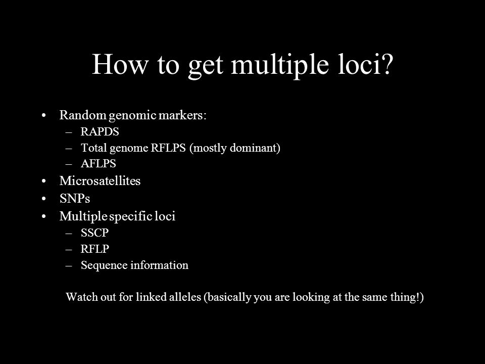
7. How to get multiple loci? Random genomic markers: –RAPDS –Total genome RFLPS (mostly dominant) –AFLPS Microsatellites SNPs Multiple specific loci –SSCP –RFLP –Sequence information Watch out for linked alleles (basically you are looking at the same thing!)

8. Sequence information Codominant Molecules have different rates of mutation, different molecules may be more appropriate for different questions 3rd base mutation Intron vs. exon Secondary tertiary structure limits Homoplasy

9. Sequence information Multiple gene genealogies=definitive phylogeny Need to ensure gene histories are comparable” partition of homogeneity test Need to use unlinked loci

10. Thermalcycler DNA template Forward primer Reverse primer

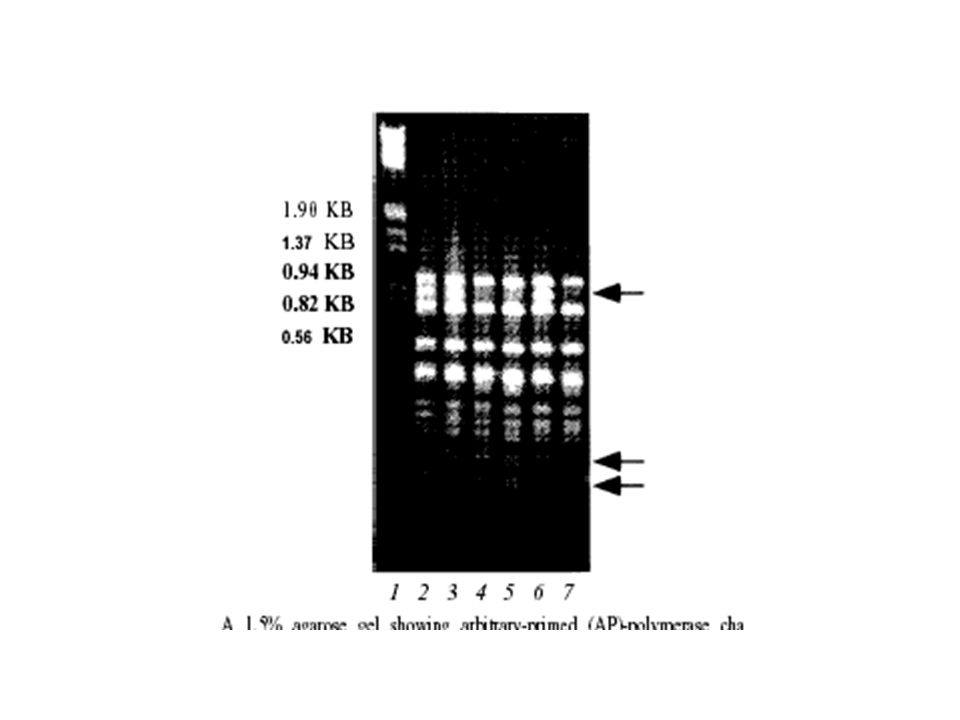
11. Gel electrophoresis to visualize PCR product Ladder (to size DNA product)

12. From DNA to genetic information (alleles are distinct DNA sequences) Presence or absence of a specific PCR amplicon (size based/ specificity of primers) Differerentiate through: –Sequencing –Restriction endonuclease –Single strand conformation polymorphism

13. Presence absence of amplicon AAAGGGTTTCCCNNNNNNNNN CCCGGGTTTAAANNNNNNNNN AAAGGGTTTCCC (primer)

14. Presence absence of amplicon AAAGGGTTTCCCNNNNNNNNN CCCGGGTTTAAANNNNNNNNN AAAGGGTTTCCC (primer)

15. Result: series of bands that are present or absent (1/0)

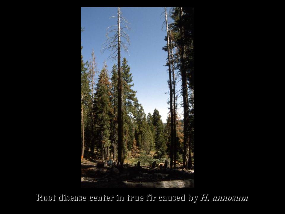
17. Root disease center in true fir caused by H. annosum

18. Ponderosa pineIncense cedar

19. Yosemite Lodge 1975 Root disease centers outlined

20. Yosemite Lodge 1997 Root disease centers outlined

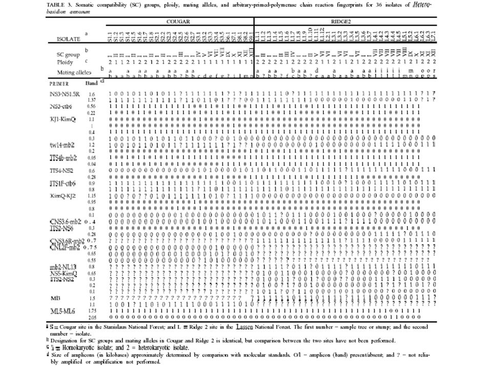
24. Are my haplotypes sensitive enough? To validate power of tool used, one needs to be able to differentiate among closely related individual Generate progeny Make sure each meiospore has different haplotype Calculate P

25. RAPD combination 1 2 1010101010 1010000000 1011101010 1010111010 1010001010 1011001010 1011110101

26. Conclusions Only one RAPD combo is sensitive enough to differentiate 4 half-sibs (in white) Mendelian inheritance? By analysis of all haplotypes it is apparent that two markers are always cosegregating, one of the two should be removed

27. AFLP Amplified Fragment Length Polymorphisms Dominant marker Scans the entire genome like RAPDs More reliable because it uses longer PCR primers less likely to mismatch Priming sites are a construct of the sequence in the organism and a piece of synthesized DNA

28. How are AFLPs generated? AGGTCGCTAAAATTTT (restriction site in red) AGGTCG CTAAATTT Synthetic DNA piece ligated –NNNNNNNNNNNNNNCTAAATTTTT Created a new PCR priming site –NNNNNNNNNNNNNNCTAAATTTTT Every time two PCR priming sitea are within 400- 1600 bp you obtain amplification

29. AFLPs are read like RAPDs (0/1)

30. Dealing with dominant anonymous multilocus markers Need to use large numbers (linkage) Repeatability Graph distribution of distances Calculate distance using Jaccard’s similarity index

31. Jaccard’s Only 1-1 and 1-0 count, 0-0 do not count 1010011 1001011 1001000

32. Jaccard’s Only 1-1 and 1-0 count, 0-0 do not count A: 1010011 AB= 0.60.4 (1-AB) B: 1001011 BC=0.50.5 C: 1001000 AC=0.20.8

33. Now that we have distances…. Plot their distribution (clonal vs. sexual)

34. Now that we have distances…. Plot their distribution (clonal vs. sexual) Analysis: –Similarity (cluster analysis); a variety of algorithms. Most common are NJ and UPGMA

35. Now that we have distances…. Plot their distribution (clonal vs. sexual) Analysis: –Similarity (cluster analysis); a variety of algorithms. Most common are NJ and UPGMA –AMOVA; requires a priori grouping

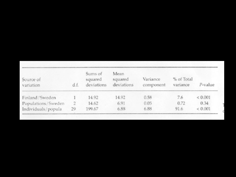
36. AMOVA groupings Individual Population Region AMOVA: partitions molecular variance amongst a priori defined groupings

37. Now that we have distances…. Plot their distribution (clonal vs. sexual) Analysis: –Similarity (cluster analysis); a variety of algorithms. Most common are NJ and UPGMA –AMOVA; requires a priori grouping –Discriminant, canonical analysis

38. Results: Jaccard similarity coefficients 0.3 0.900.920.94 0.960.98 1.00 0 0.1 0.2 0.4 0.5 0.6 0.7 Coefficient Frequency P. nemorosa P. pseudosyringae: U.S. and E.U. 0.3 Coefficient 0.900.920.940.960.981.00 0 0.1 0.2 0.4 0.5 0.6 0.7 Frequency

39. 0.90.910.920.930.940.950.960.970.980.99 Pp U.S. Pp E.U. 0.0 0.1 0.2 0.3 0.4 0.5 0.6 Jaccard coefficient of similarity 0.7 P. pseudosyringae genetic similarity patterns are different in U.S. and E.U.

40. P. nemorosa P. ilicis P. pseudosyringae Results: P. nemorosa

41. Results: P. pseudosyringae P. nemorosa P. ilicis P. pseudosyringae = E.U. isolate

42. Now that we have distances…. Plot their distribution (clonal vs. sexual) Analysis: –Similarity (cluster analysis); a variety of algorithms. Most common are NJ and UPGMA –AMOVA; requires a priori grouping –Discriminant, canonical analysis –Frequency: does allele frequency match expected (hardy weinberg), F or Wright’s statistsis

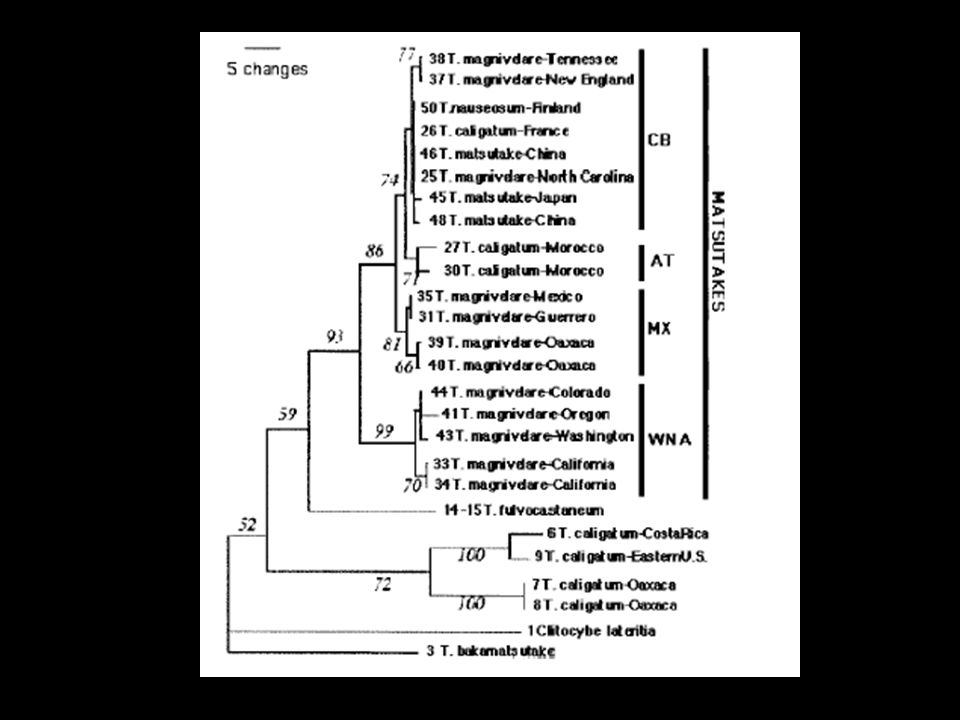
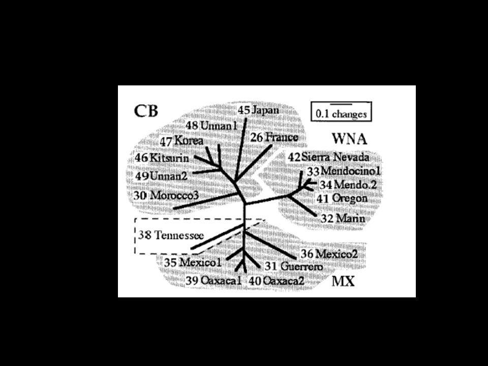
43. The “scale” of disease Dispersal gradients dependent on propagule size, resilience, ability to dessicate, NOTE: not linear Important interaction with environment, habitat, and niche availability. Examples: Heterobasidion in Western Alps, Matsutake mushrooms that offer example of habitat tracking Scale of dispersal (implicitely correlated to metapopulation structure)---

44. Have we sampled enough? Resampling approaches Saturation curves –A total of 30 polymorphic alleles –Our sample is either 10 or 20 –Calculate whether each new sample is characterized by new alleles

45. Saturation curves 1 2 3 4 5 6 7 8 9 10 11 12 13 14 15 16 17 18 19 20 No Of New alleles

46. If we have codominant markers how many do I need IDENTITY tests = probability calculation based on allele frequency… Multiplication of frequencies of alleles 10 alleles at locus 1 P1=0.1 5 alleles at locus 2 P2=0,2 Total P= P1*P2=0.02

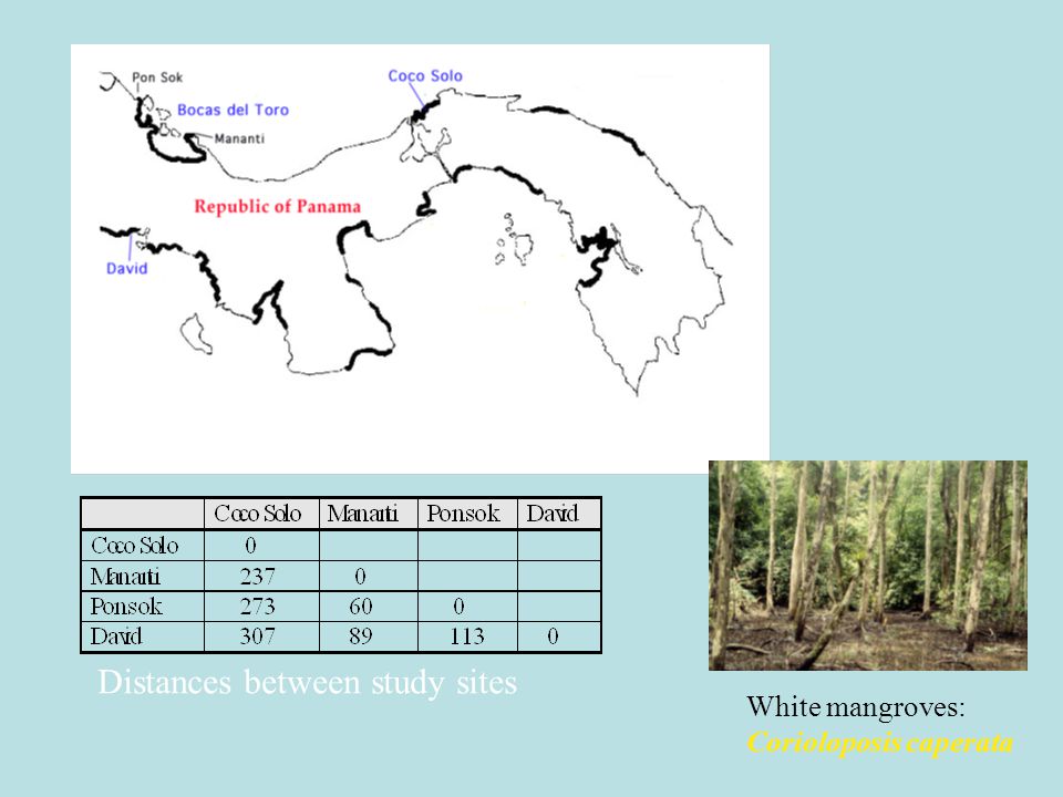
47. White mangroves: Corioloposis caperata

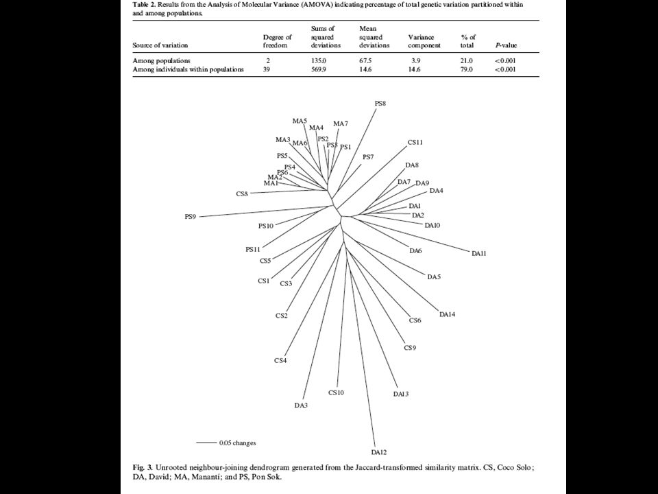
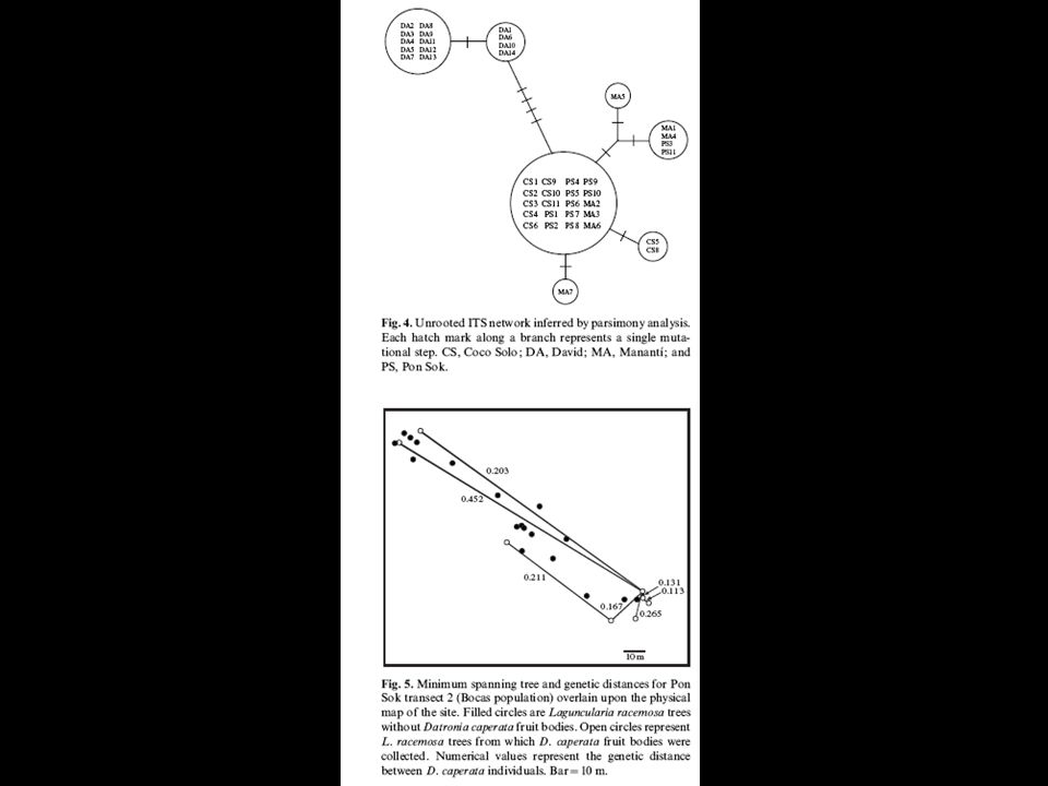
51. White mangroves: Corioloposis caperata Distances between study sites

52. Coriolopsis caperata on Laguncularia racemosa Forest fragmentation can lead to loss of gene flow among previously contiguous populations. The negative repercussions of such genetic isolation should most severely affect highly specialized organisms such as some plant- parasitic fungi. AFLP study on single spores

54. Using DNA sequences Obtain sequence Align sequences, number of parsimony informative sites Gap handling Picking sequences (order) Analyze sequences (similarity/parsimony/exhaustive/bayesian Analyze output; CI, HI Bootstrap/decay indices

55. Using DNA sequences Testing alternative trees: kashino hasegawa Molecular clock Outgroup Spatial correlation (Mantel) Networks and coalescence approaches

56. Pacifico Caribe

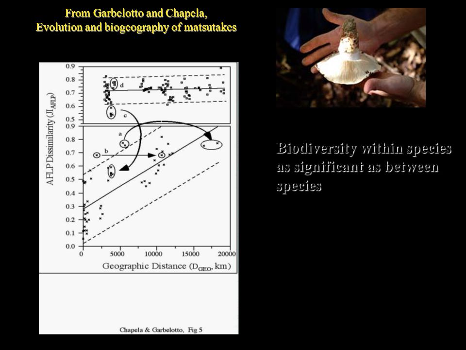
61. From Garbelotto and Chapela, Evolution and biogeography of matsutakes Biodiversity within species as significant as between species