1. 1 Econ 240A Power 6

2. 2 The Challenger Disaster l http://onlineethics.org/moral/boi sjoly/RB-intro.html http://onlineethics.org/moral/boi sjoly/RB-intro.html

3. 3 The Challenger l The issue is whether o-ring failure on prior 24 prior launches is temperature dependent l They were considering launching Challenger at about 32 degrees l What were the temperatures of prior launches?

4. 4 Challenger Launch Only 4 launches Between 50 and 64 degrees

5. 5 Challenger l Divide the data into two groups 12 low temperature launches, 53- 70 degrees 12 high temperature launches, 70- 81 degrees

6. TemperatureO-Ring Failure 53Yes 57Yes 58Yes 63Yes 66No 67NO 67No 67No 68No 69No 70No 70Yes

7. TemperatureO-Ring Failure 70Yes 70No 72No 73No 75Yes 75No 76No 76No 78No 79No 80No 81No

8. 8 Probability of O-Ring Failure Conditional On Temperature, P/T l P/T=#of Yeses/# of Launches at low temperature P/T=#of O-Ring Failures/# of Launches at low temperature Pˆ = k(low)/n(low) = 5/12 = 0.41 l P/T=#of Yeses/# of Launches at high temperature Pˆ = k(high)/n(high) = 2/12 = 0.17

9. 9 Are these two rates significantly different? l Dispersion: p*(1-p)/n Low: [p*(1-p)/n] 1/2 = [0.41*0.59/12] 1/2 =0.14 High: [p*(1-p)/n] 1/2 = [0.17*0.83/12] 1/2 =0.11 l So.41 -.17 =.24 is 1.7 to 2.2 standard deviations apart? Is that enough to be statistically significant?

10. 10 Interval Estimation and Hypothesis Testing

11. 11 Outline l Interval Estimation l Hypothesis Testing l Decision Theory

12. 0

13. 0

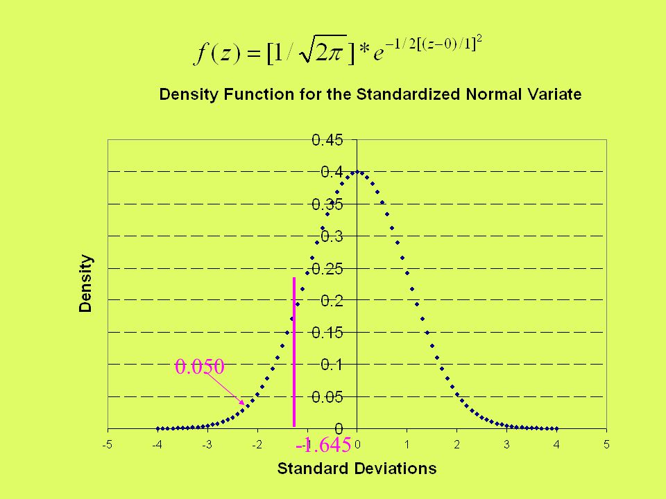
14. -1.645 0.050

15. 15 a Z value of 1.96 leads to an area of 0.475, leaving 0.025 in the Upper tail

16. 16 Interval Estimation l The conventional approach is to choose a probability for the interval such as 95% or 99%

17. 17 So z values of -1.96 and 1.96 leave 2.5% in each tail

18. -1.96 2.5% 1.96

19. 19 http://www.sfgate.com/election/races/2003/10/07/map.shtml Two Californias

20. 20 Interval Estimation l Sample mean example: Monthly Rate of Return, UC Stock Index Fund, Sept. 1995 - Aug. 2004 number of observations: 108 sample mean: 0.842 sample standard deviation: 4.29 Student’s t-statistic degrees of freedom: 107

21. Sample Mean 0.842

22. 22 Appendix B Table 4 p. B-9 2.5 % in the upper tail

23. 23 Interval Estimation l 95% confidence interval l substituting for t

24. 24 Interval Estimation l Multiplying all 3 parts of the inequality by 0.413 l subtracting.842 from all 3 parts of the inequality,

25. 25 Interval Estimation An Inference about E(r) l And multiplying all 3 parts of the inequality by -1, which changes the sign of the inequality l So, the population annual rate of return on the UC Stock index lies between 19.9% and 0.2% with probability 0.95, assuming this rate is not time varying

26. 26 Hypothesis Testing

27. 27 Hypothesis Testing: 4 Steps l Formulate all the hypotheses l Identify a test statistic l If the null hypothesis were true, what is the probability of getting a test statistic this large? l Compare this probability to a chosen critical level of significance, e.g. 5%

28. 28

29. -1.645 5 % lower tail Step #4: compare the probability for the test statistic(z= -1.33) to the chosen critical level (z=-1.645)

30. 30 Decision Theory

31. l Inference about unknown population parameters from calculated sample statistics are informed guesses. So it is possible to make mistakes. The objective is to follow a process that minimizes the expected cost of those mistakes. l Types of errors involved in accepting or rejecting the null hypothesis depends on the true state of nature which we do not know at the time we are making guesses about it.

32. Decision Theory l For example, consider a possible proposition for bonds to finance dams, and the null hypothesis that the proportion that would vote yes would be 0.4999 (or less), i.e. p ~ 0.5. The alternative hypothesis was that this proposition would win i.e., p >= 0.5.

33. Decision Theory l If we accept the null hypothesis when it is true, there is no error. If we reject the null hypothesis when it is false there is no error.

34. 34 Decision theory l If we reject the null hypothesis when it is true, we commit a type I error. If we accept the null when it is false, we commit a type II error.

35. Decision Accept null Reject null True State of Nature p = 0.4999 H 2 o Bonds lose P >= 0.5 Bonds win No Error Type I error No Error Type II error

36. Decision Theory The size of the type I error is the significance level or probability of making a type I error,  The size of the type II error is the probability of making a type II error, 

37. 37 Decision Theory We could choose to make the size of the type I error smaller by reducing  for example from 5 % to 1 %. But, then what would that do to the type II error?

38. Decision Accept null Reject null True State of Nature p = 0.4999P >= 0.5 No Error 1 -  Type I error  No Error 1 -  Type II error 

39. Decision Theory l There is a tradeoff between the size of the type I error and the type II error.

40. 40 Decision Theory l This tradeoff depends on the true state of nature, the value of the population parameter we are guessing about. To demonstrate this tradeoff, we need to play what if games about this unknown population parameter.

41. 41 What is at stake? l Suppose you are for Water Bonds. l What does the water bonds camp want to believe about the true population proportion p? they want to reject the null hypothesis, p=0.4999 they want to accept the alternative hypothesis, p>=0.5

42. Cost of Type I and Type II Errors l The best thing for the water bonds camp is to lean the other way from what they want l The cost to them of a type I error, rejecting the null when it is true (i.e believing the bonds will pass) is high: over- confidence at the wrong time. l Expected Cost E(C) = C I high (type I error)*P(type I error) + C II low (type II error)*P(type II error)

43. 43 Costs in Water Bond Camp l Expected Cost E(C) = C I high (type I error)*P(type I error) + C II low (type II error)*P(type II error) E(C) = C I high (type I error)*  C II low (type II error)*  l Recommended Action: make probability of type I error small, i.e. run scared so chances of losing stay small

44. Decision Accept null Reject null True State of Nature p = 0.499 Bonds lose P >= 0.5 Bonds win No Error 1 -  Type I error  C(I) No Error 1 -  Type II error  C(II) E[C] = C(I)*  + C(II)*  Bonds: C(I) is large so make  small

45. 45 How About Costs to the Bond Opponents Camp ? l What do they want? l They want to accept the null, p=0.499 i.e. Bonds lose l The opponents camp should lean against what they want l The cost of accepting the null when it is false is high to them, so C(II) is high

46. 46 Costs in the opponents Camp l Expected Cost E(C) = C low (type I error)*P(type I error) + C high (type II error)*P(type II error) E(C) = C low (type I error)*  C high (type II error)*  l Recommended Action: make probability of type II error small, i.e. make the probability of accepting the null when it is false small

47. Decision Accept null Reject null True State of Nature p = 0.499 Bonds lose P >=0.5 Bonds win No Error 1 -  Type I error  C(I) No Error 1 -  Type II error  C(II) E[C] = C(I)*  + C(II)*  Opponents: C(II) is large so make  small

48. Decision Theory Example If we set the type I error,  to 1%, then from the normal distribution (Table 3), the standardized normal variate z will equal 2.33 for 1% in the upper tail. For a sample size of 1000, where p~0.5 from null

49. 49 Decision theory example So for this poll size of 1000, with p=0.5 under the null hypothesis, given our choice of the type I error of size 1%, which determines the value of z of 2.33, we can solve for a

50. 2.33 1 %

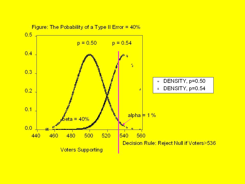
51. Decision Theory Example l So if 53.7% of the polling sample, or 0.5368*1000=537 say they will vote for water bonds, then we reject the null of p=0.499, i.e the null that the bond proposition will lose

52. 52 Decision Theory Example l But suppose the true value of p is 0.54, and we use this decision rule to reject the null if 537 voters are for the bonds, but accept the null (of p=0.499, false if p=0.54) if this number is less than 537. What is the size of the type II error?

54. Decision Theory Example What is the value of the type II error,  if the true population proportion is p = 0.54? l Recall our decision rule is based on a poll proportion of 0.536 or 536 for Bonds l z(beta) = (0.536 – p)/[p*(1-p)/n] 1/2 l Z(beta) = (0.536 – 0.54)/[.54*.46/1000] 1/2 l Z(beta) = -0.253

55. Calculation of Beta

56. Beta Versus p (true) p 

57. Power of the Test p 1 - 

58. Power of the Test p 1 -  Ideal

59. Decision Accept null Reject null True State of Nature p = 0.499P >= 0.5 No Error 1 -  Type I error  No Error 1 -  Type II error 

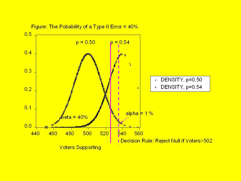
60. 60 Tradeoff Between  and  l Suppose the type I error is 5% instead of 1%; what happens to the type II error?

61. 61 Tradeoff If  then the Z value in our example is 1.645 instead of 2.33 and the decision rule is reject the null if 526 voters are for water bonds.