Download presentation
Presentation is loading. Please wait.

1
1 Econ 240A Power 6

2
2 Interval Estimation and Hypothesis Testing

3
3 Outline l Interval Estimation l Hypothesis Testing l Decision Theory

4
4 How good was last week’s LA Times Poll? l Oct 1, 2003 LA Times

5
5 Power 4

6
6 The Los Angeles Times Poll l In a sample of approximately 2000 people, 56% indicate they will vote to recall Governor Davis l If the poll is an accurate reflection or subset of the population of voters next Tuesday, what is the expected proportion that will vote for the recall? l How much uncertainty is in that expectation? Power 4

7
LA Times Poll l The estimated proportion, from the sample, that will vote for recall is: l where is 0.56 or 56% l k is the number of “successes”, the number of people sampled who are for recall, approximately 1,120 l n is the size of the sample, 2000 Power 4

8
LA Times Poll l What is the expected proportion of voters next Tuesday that will vote for recall? l = E(k)/n = np/n = p, where from the binomial distribution, E(k) = np l So if the sample is representative of voters and their preferences, 56% should vote for recall next Tuesday Power 4
/n = np/n = p, where from the binomial distribution, E(k) = np l So if the sample is representative of voters and their preferences, 56% should vote for recall next Tuesday Power 4.")
9
LA Times Poll l How much dispersion is in this estimate, i.e. as reported in newspapers, what is the margin of sampling error? l The margin of sampling error is calculated as the standard deviation or square root of the variance in l = VAR(k)/n 2 = np(1-p)/n 2 =p(1- p)/n l and using 0.56 as an estimate of p, l = 0.56*0.44/2000 =0.0001 Power 4
/n 2 = np(1-p)/n 2 =p(1- p)/n l and using 0.56 as an estimate of p, l = 0.56*0.44/2000 = Power 4.")
10
10 Interval Estimation l Based on the Poll of 56% for recall, what was the probability that the fraction, p, voting for recall would exceed 50%, i.e. lie between 0.5 and 1.0? l The standardized normal variate, z =

11
11 Interval estimation l Why can we use the normal distribution? l Where does the formula for z come from?

12
Solving for p:.01*z = 0.56 - p p = 0.56 -.01*z and substituting for p: and subtracting 0.56 from each of the 3 parts of this inequality:

13
And multiplying by -100, which changes the signs of the inequality: And using the standardized normal distribution, this probability equals ….

14
6-44

15
6

16
16 Interval Estimation l So by last Wednesday, Arnold’s camp knew that if the “big mo’” did not shift, they were in fat city… l Rather than using values a=0.5, and b=1 for the unknown parameter p, the fraction that would vote for Swarzenegger, the conventional approach is to choose a probability for the interval such as 95% or 99%

17
17 So z values of -1.96 and 1.96 leave 2.5% in each tail

18
-1.96 2.5% 1.96

19
Substituting for z And multiplying all three parts of the inequality by 0.01

20
And subtracting 0.56 from all three parts of the inequality And multiplying by -1, which changes the signs of the inequality: So a 95% confidence interval based on the poll, predicted a recall vote between 54% and 58%, an inference about the unknown parameter p. Z values of -2.575 and 2.575 leave 1/2% in each tail. You might calculate a 99% confidence interval for the poll.

21
21 Based on the Santa Barbara News-Press, with about 52% of the vote counted, recall was 55% yes

22
22 http://www.sfgate.com/election/races/2003/10/07/map.shtml

23
23 Interval Estimation l Sample mean example: Monthly Rate of Return, UC Stock Index Fund, Sept. 1995 - Aug. 2003 number of observations: 96 sample mean: 0.816 sample standard deviation: 4.46 Student’s t-statistic degrees of freedom: 95

24
Sample mean 0.816

25
25 Appendix B Table 4 p. B-9 2.5 % in the upper tail

26
26 Interval Estimation l 95% confidence interval l substituting for t

27
27 Interval Estimation l Multiplying all 3 parts of the inequality by 0.155 l subtracting.816 from all 3 parts of the inequality,

28
28 Interval Estimation An Inference about E(r) l And multiplying all 3 parts of the inequality by -1, which changes the sign of the inequality l So, the population annual rate of return on the UC Stock index lies between 13.4% and 6.1% with probability 0.95, assuming this rate is not time varying
 l And multiplying all 3 parts of the inequality by -1, which changes the sign of the inequality l So, the population annual rate of return on the UC Stock index lies between 13.4% and 6.1% with probability 0.95, assuming this rate is not time varying")
29
29 Hypothesis Testing

30
30 Hypothesis Testing: 4 Steps l Formulate all the hypotheses l Identify a test statistic l If the null hypothesis were true, what is the probability of getting a test statistic this large? l Compare this probability to a chosen critical level of significance, e.g. 5%

31
31 Hypothesis Test Example l Last Week’s LA Times Poll on Recall a l Step #1: null, i.e. the maintained, hypothesis: true proportion for recall is 50% H 0 : p = 0.5; the alternative hypothesis is that the true population proportion supporting recall is greater than 50%, H a : p>0.5

32
32 Hypothesis Test Example l Step #2: test statistic: standardized normal variate z l Step #3: Critical level for rejecting the null hypothesis: e.g. 5% in upper tail; alternative 1% in upper tail

33
33

34
6 1.645 5 % upper tail Sample statistic Step #4: compare the probability for the test statistic(z=6) to the chosen critical level(z=1.645)
 to the chosen critical level(z=1.645)")
35
35 Hypothesis Test Example l So reject the null hypothesis

36
36 Decision Theory

37
l Inference about unknown population parameters from calculated sample statistics are informed guesses. So it is possible to make mistakes. The objective is to follow a process that minimizes the expected cost of those mistakes. l Types of errors involved in accepting or rejecting the null hypothesis depends on the true state of nature which we do not know at the time we are making guesses about it.

38
Decision Theory l For example, consider the LA Times poll of Oct. 1, and the null hypothesis that the proportion that would vote for recall the following week was 0.5, i.e. p = 0.5. The alternative hypothesis was that this proportion was greater than 0.5, p > 0.5. Last week, no one knew which was right, but guesses could be made based on the poll.

39
Decision Theory l If we accept the null hypothesis when it is true, there is no error. If we reject the null hypothesis when it is false there is no error. l If we reject the null hypothesis when it is true, we commit a type I error. If we accept the null when it is false, we commit a type II error.

40
Decision Accept null Reject null True State of Nature p = 0.5P > 0.5 No Error Type I error No Error Type II error

41
Decision Theory The size of the type I error is the significance level or probability of making a type I error, The size of the type II error is the probability of making a type II error, We could choose to make the size of the type I error smaller by reducing for example from 5 % to 1 %. But, then what would that do to the type II error?

42
Decision Accept null Reject null True State of Nature p = 0.5P > 0.5 No Error 1 - Type I error No Error 1 - Type II error

43
Decision Theory l There is a tradeoff between the size of the type I error and the type II error. l This tradeoff depends on the true state of nature, the value of the population parameter we are guessing about. To demonstrate this tradeoff, we need to play what if games about this unknown population parameter.

44
44 What is at stake? l Suppose last Wednesday you were in Arnold’s camp. l What does the Arnold camp want to believe about the true population proportion p? they want to reject the null hypothesis, p=0.5 they want to accept the alternative hypothesis, p>0.5

45
Cost of Type I and Type II Errors l The best thing for the Arnold camp is to lean the other way from what they want l The cost to them of a type I error, rejecting the null when it is true is high. They might relax at the wrong time. l Expected Cost E(C) = C high (type I error)*P(type I error) + C low (type II error)*P(type II error)
 = C high (type I error)*P(type I error) + C low (type II error)*P(type II error).")
46
46 Costs in Arnold’s Camp l Expected Cost E(C) = C high (type I error)*P(type I error) + C low (type II error)*P(type II error) E(C) = C high (type I error)* C low (type II error)* l Recommended Action: make probability of type I error small, i.e. don’t be eager to reject the null

47
Decision Accept null Reject null True State of Nature p = 0.5P > 0.5 No Error 1 - Type I error C(I) No Error 1 - Type II error C(II) E[C] = C(I)* + C(II)* Arnold: C(I) is large so make small
![Decision Accept null Reject null True State of Nature p = 0.5P > 0.5 No Error 1 - Type I error C(I) No Error 1 - Type II error C(II) E[C] = C(I)* + C(II)* Arnold: C(I) is large so make small](http://images.slideplayer.com/16/5071732/slides/slide_47.jpg "Decision Accept null Reject null True State of Nature p = 0.5P > 0.5 No Error 1 - Type I error C(I) No Error 1 - Type II error C(II) E[C] = C(I)* + C(II)* Arnold: C(I) is large so make small")
48
48 How About Costs to the Davis Camp on Oct 1? l What do they want? l They do not want to reject the null, p=0.5 l The Davis camp should lean against what they want l The cost of accepting the null when it is false is high to them, so C(II) is high
 is high.")
49
49 Costs in the Davis Camp l Expected Cost E(C) = C low (type I error)*P(type I error) + C high (type II error)*P(type II error) E(C) = C low (type I error)* C high (type II error)* l Recommended Action: make probability of type II error small, i.e. make the probability of accepting the null when it is false small

50
Decision Accept null Reject null True State of Nature p = 0.5P > 0.5 No Error 1 - Type I error C(I) No Error 1 - Type II error C(II) E[C] = C(I)* + C(II)* Davis: C(II) is large so make small
![Decision Accept null Reject null True State of Nature p = 0.5P > 0.5 No Error 1 - Type I error C(I) No Error 1 - Type II error C(II) E[C] = C(I)* + C(II)* Davis: C(II) is large so make small](http://images.slideplayer.com/16/5071732/slides/slide_50.jpg "Decision Accept null Reject null True State of Nature p = 0.5P > 0.5 No Error 1 - Type I error C(I) No Error 1 - Type II error C(II) E[C] = C(I)* + C(II)* Davis: C(II) is large so make small")
51
Decision Theory Example If we set the type I error, to 1%, then from the normal distribution (Table 3), the standardized normal variate z will equal 2.33 for 1% in the upper tail. So for this poll size of 2000, with p=0.5 under the null hypothesis, given our choice of the type I error of size 1%, which determines the value of z of 2.33, we can solve for a

52
2.33 1 %

53
Decision Theory Example l So if 52.6% of the polling sample, or 0.526*2000=1052 say they will recall, then we reject the null of p=0.5. l But suppose the true value of p is 0.54, and we use this decision rule to reject the null if 1052 voters are for recall, but accept the null (assumed false if p=0.54) if this number is less than 1052. What is the size of the type II error?
 if this number is less than What is the size of the type II error .")
54
Reject NullAccept Null 1052 alpha = 1 % ?

55
Decision Theory Example What is the value of the type II error, if the true population proportion is p = 0.54? l Recall our decision rule is based on a poll proportion of 0.526 or 1052 for recall l z(beta) = (0.526 – p)/[p*(1-p)/n] 1/2 l Z(beta) = (0.526 – 0.54)/[.54*.46/2000] 1/2 l Z(beta) = -1.256
 = (0.526 – p)/[p*(1-p)/n] 1/2 l Z(beta) = (0.526 – 0.54)/[.54*.46/2000] 1/2 l Z(beta) =")
56
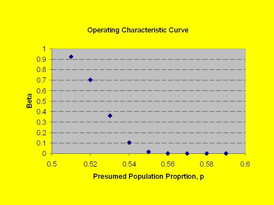
Decision Theory Example

58
Ideal power function

Similar presentations

 Parameter Estimation of PDF and Fitting a Distribution Function.>")


