Download presentation
Presentation is loading. Please wait.

2
Recursive Bayes Filtering Advanced AI Wolfram Burgard

3
Tutorial Goal To familiarize you with probabilistic paradigm in robotics Basic techniques Advantages Pitfalls and limitations Successful Applications Open research issues

4
Robotics Yesterday

5
Robotics Today

6
Robotics Tomorrow?

8
Tasks to be Solved by Robots Planning Perception Modeling Localization Interaction Acting Manipulation Cooperation ...

9
Current Trends in Robotics Robots are moving away from factory floors to Entertainment, toys Personal services Medical, surgery Industrial automation (mining, harvesting, …) Hazardous environments (space, underwater)
 Hazardous environments (space, underwater)")
10
RoboCup

11
Physical Agents are Inherently Uncertain Uncertainty arises from four major factors: Environment stochastic, unpredictable Robot stochastic Sensor limited, noisy Models inaccurate

12
Example: Museum Tour-Guide Robots Rhino, 1997 Minerva, 1998

13
Rhino (Univ. Bonn + CMU, 1997) W. Burgard, A.B. Cremers, D. Fox, D. Hähnel, G. Lakemeyer, D. Schulz, W. Steiner, S. Thrun

14
Minerva (CMU + Univ. Bonn, 1998) Minerva S. Thrun, M. Beetz, M. Bennewitz, W. Burgard, A.B. Cremers, F. Dellaert, D. Fox, D. Hähnel, C. Rosenberg, N. Roy, J. Schulte, D. Schulz

15
Technical Challenges Navigation Environment crowded, unpredictable Environment unmodified “Invisible” hazards Walking speed or faster High failure costs Interaction Individuals and crowds Museum visitors’ first encounter Age 2 through 99 Spend less than 15 minutes

16
Nature of Sensor Data Odometry Data Range Data

17
Probabilistic Techniques for Physical Agents Key idea: Explicit representation of uncertainty using the calculus of probability theory Perception = state estimation Action = utility optimization

18
Advantages of Probabilistic Paradigm Can accommodate inaccurate models Can accommodate imperfect sensors Robust in real-world applications Best known approach to many hard robotics problems

19
Pitfalls Computationally demanding False assumptions Approximate

20
Outline Introduction Probabilistic State Estimation Robot Localization Probabilistic Decision Making Planning Between MDPs and POMDPs Exploration Conclusions

21
Pr(A) denotes probability that proposition A is true. Axioms of Probability Theory
 denotes probability that proposition A is true. Axioms of Probability Theory")
22
A Closer Look at Axiom 3 B

23
Using the Axioms

24
Discrete Random Variables X denotes a random variable. X can take on a finite number of values in {x 1, x 2, …, x n }. P(X=x i ), or P(x i ), is the probability that the random variable X takes on value x i. P( ) is called probability mass function. E.g..
, or P(x i ), is the probability that the random variable X takes on value x i. P( ) is called probability mass function. E.g...")
25
Continuous Random Variables X takes on values in the continuum. p(X=x), or p(x), is a probability density function. E.g. x p(x)
, or p(x), is a probability density function. E.g. x p(x).")
26
Joint and Conditional Probability P(X=x and Y=y) = P(x,y) If X and Y are independent then P(x,y) = P(x) P(y) P(x | y) is the probability of x given y P(x | y) = P(x,y) / P(y) P(x,y) = P(x | y) P(y) If X and Y are independent then P(x | y) = P(x)
 = P(x,y) If X and Y are independent then P(x,y) = P(x) P(y) P(x | y) is the probability of x given y P(x | y) = P(x,y) / P(y) P(x,y) = P(x | y) P(y) If X and Y are independent then P(x | y) = P(x)")
27
Law of Total Probability, Marginals Discrete caseContinuous case

28
Bayes Formula

29
Normalization Algorithm:

30
Conditioning Total probability: Bayes rule and background knowledge:

31
Simple Example of State Estimation Suppose a robot obtains measurement z What is P(open|z)?
")
32
Causal vs. Diagnostic Reasoning P(open|z) is diagnostic. P(z|open) is causal. Often causal knowledge is easier to obtain. Bayes rule allows us to use causal knowledge: count frequencies!
 is causal. Often causal knowledge is easier to obtain. Bayes rule allows us to use causal knowledge: count frequencies!.")
33
Example P(z|open) = 0.6P(z| open) = 0.3 P(open) = P( open) = 0.5 z raises the probability that the door is open.
 = 0.6P(z| open) = 0.3 P(open) = P( open) = 0.5 z raises the probability that the door is open.")
34
Combining Evidence Suppose our robot obtains another observation z 2. How can we integrate this new information? More generally, how can we estimate P(x| z 1...z n ) ?
 .")
35
Recursive Bayesian Updating Markov assumption: z n is independent of z 1,...,z n-1 if we know x.

36
Example: Second Measurement P(z 2 |open) = 0.5P(z 2 | open) = 0.6 P(open|z 1 )= 2/3 z 2 lowers the probability that the door is open.
 = 0.5P(z 2 | open) = 0.6 P(open|z 1 )= 2/3 z 2 lowers the probability that the door is open.")
37
A Typical Pitfall Two possible locations x 1 and x 2 P(x 1 )= 1-P(x 2 )= 0.99 P(z|x 2 )=0.09 P(z|x 1 )=0.07
= 1-P(x 2 )= 0.99 P(z|x 2 )=0.09 P(z|x 1 )=0.07")
38
Actions Often the world is dynamic since actions carried out by the robot, actions carried out by other agents, or just the time passing by change the world. How can we incorporate such actions?

39
Typical Actions The robot turns its wheels to move The robot uses its manipulator to grasp an object Plants grow over time… Actions are never carried out with absolute certainty. In contrast to measurements, actions generally increase the uncertainty.

40
Modeling Actions To incorporate the outcome of an action u into the current “belief”, we use the conditional pdf P(x|u,x’) This term specifies the pdf that executing u changes the state from x’ to x.
 This term specifies the pdf that executing u changes the state from x’ to x.")
41
Example: Closing the door

42
State Transitions P(x|u,x’) for u = “close door”: If the door is open, the action “close door” succeeds in 90% of all cases.
 for u = close door : If the door is open, the action close door succeeds in 90% of all cases.")
43
Integrating the Outcome of Actions Continuous case: Discrete case:

44
Example: The Resulting Belief

45
Bayes Filters: Framework Given: Stream of observations z and action data u: Sensor model P(z|x). Action model P(x|u,x’). Prior probability of the system state P(x). Wanted: Estimate of the state X of a dynamical system. The posterior of the state is also called Belief:
. Prior probability of the system state P(x). Wanted: Estimate of the state X of a dynamical system. The posterior of the state is also called Belief:.")
46
Markov Assumption Underlying Assumptions Static world Independent noise Perfect model, no approximation errors X t-1 XtXt X t+1 Z t-1 ZtZt Z t+1 u t-1 utut

47
Bayes Filters Bayes z = observation u = action x = state Markov Total prob.

48
Bayes Filter Algorithm 1. Algorithm Bayes_filter( Bel(x),d ): 2. 0 3. if d is a perceptual data item z then 4. For all x do 5. 6. 7. For all x do 8. 9. else if d is an action data item u then 10. For all x do 11. 12. return Bel’(x)
.")
49
Bayes Filters are Familiar! Kalman filters Particle filters Hidden Markov models Dynamic Bayes networks Partially Observable Markov Decision Processes (POMDPs)
.")
50
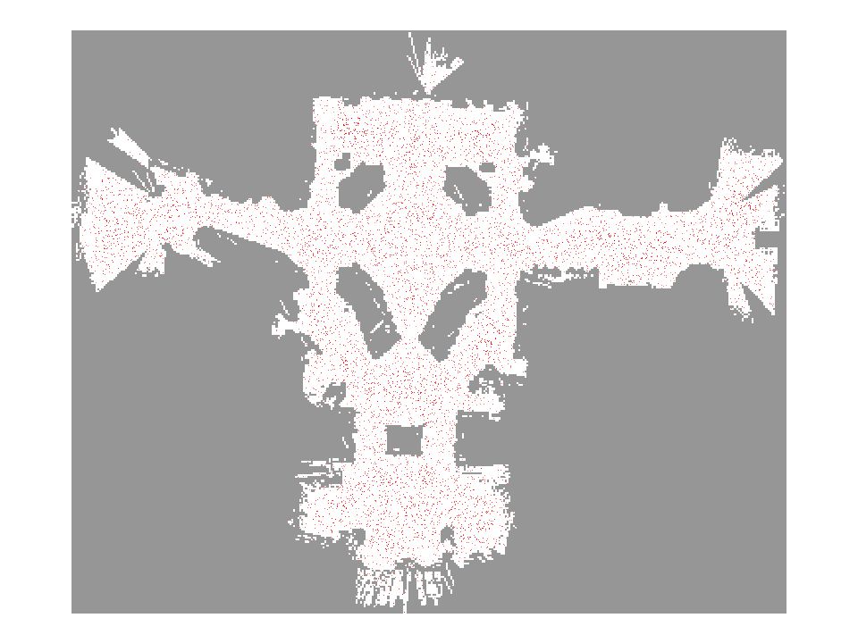
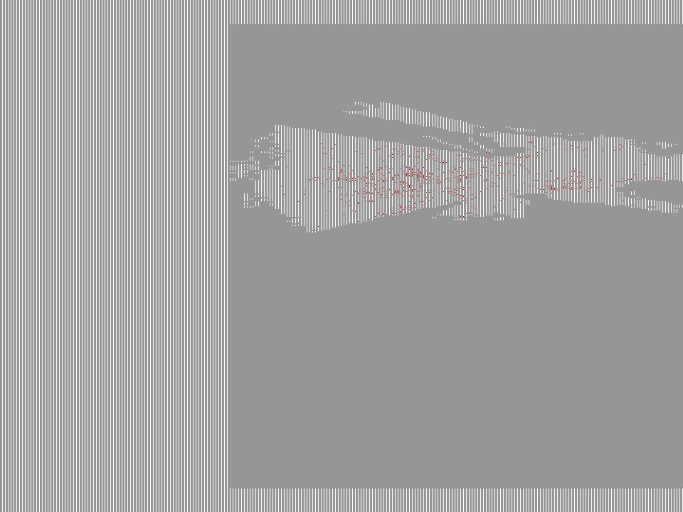
Application to Door State Estimation Estimate the opening angle of a door and the state of other dynamic objects using a laser-range finder from a moving mobile robot and based on Bayes filters.

51
Result

52
Lessons Learned Bayes rule allows us to compute probabilities that are hard to assess otherwise. Under the Markov assumption, recursive Bayesian updating can be used to efficiently combine evidence. Bayes filters are a probabilistic tool for estimating the state of dynamic systems.

53
Tutorial Outline Introduction Probabilistic State Estimation Localization Probabilistic Decision Making Planning Between MDPs and POMDPs Exploration Conclusions

54
The Localization Problem Given Map of the environment. Sequence of sensor measurements. Wanted Estimate of the robot’s position. Problem classes Position tracking Global localization Kidnapped robot problem (recovery) “Using sensory information to locate the robot in its environment is the most fundamental problem to providing a mobile robot with autonomous capabilities.” [Cox ’91]
 Using sensory information to locate the robot in its environment is the most fundamental problem to providing a mobile robot with autonomous capabilities. [Cox ’91].")
55
Representations for Bayesian Robot Localization Discrete approaches (’95) Topological representation (’95) uncertainty handling (POMDPs) occas. global localization, recovery Grid-based, metric representation (’96) global localization, recovery Multi-hypothesis (’00) multiple Kalman filters global localization, recovery Particle filters (’99) sample-based representation global localization, recovery Kalman filters (late-80s?) Gaussians approximately linear models position tracking AI Robotics
 global localization, recovery Multi-hypothesis (’00) multiple Kalman filters global localization, recovery Particle filters (’99) sample-based representation global localization, recovery Kalman filters (late-80s ) Gaussians approximately linear models position tracking AI Robotics.")
56
Localization with Bayes Filters map m s’ a p(s|a,s’,m) a s’ laser datap(o|s,m) observation o
 a s’ laser datap(o|s,m) observation o")
57
Localization with Bayes Filters Motion: Perception: … is optimal under the Markov assumption

58
What is the Right Representation? Kalman filters Multi-hypothesis tracking Grid-based representations Topological approaches Particle filters

59
Gaussians -- Univariate Multivariate

60
59 Kalman Filters Estimate the state of processes that are governed by the following linear stochastic difference equation. The random variables v t and w t represent the process measurement noise and are assumed to be independent, white and with normal probability distributions.

61
[Schiele et al. 94], [Weiß et al. 94], [Borenstein 96], [Gutmann et al. 96, 98], [Arras 98] Kalman Filters
![[Schiele et al. 94], [Weiß et al. 94], [Borenstein 96], [Gutmann et al.](http://images.slideplayer.com/15/4559595/slides/slide_61.jpg "96, 98], [Arras 98] Kalman Filters.")
62
Kalman Filter Algorithm 1. Algorithm Kalman_filter( <, d ): 2. If d is a perceptual data item z then 3. 4. 5. 6. Else if d is an action data item u then 7. 8. 9. Return <

63
Non-linear Systems Very strong assumptions: Linear state dynamics Observations linear in state What can we do if system is not linear? Linearize it: EKF Compute the Jacobians of the dynamics and observations at the current state. Extended Kalman filter works surprisingly well even for highly non-linear systems.

64
[Gutmann et al. 96, 98]: Match LRF scans against map Highly successful in RoboCup mid-size league Kalman Filter-based Systems (1) Courtesy of S. Gutmann
 Courtesy of S. Gutmann.")
65
Kalman Filter-based Systems (2) Courtesy of S. Gutmann
 Courtesy of S. Gutmann")
66
[Arras et al. 98]: Laser range-finder and vision High precision (<1cm accuracy) Kalman Filter-based Systems (3) Courtesy of K. Arras
 Kalman Filter-based Systems (3) Courtesy of K. Arras.")
67
Localization Algorithms - Comparison Kalman filter SensorsGaussian PosteriorGaussian Efficiency (memory) ++ Efficiency (time)++ Implementation+ Accuracy++ Robustness- Global localization No
 ++ Efficiency (time)++ Implementation+ Accuracy++ Robustness- Global localization No")
68
[Cox 92], [Jensfelt, Kristensen 99] Multi- hypothesis Tracking
![[Cox 92], [Jensfelt, Kristensen 99] Multi- hypothesis Tracking](http://images.slideplayer.com/15/4559595/slides/slide_68.jpg "[Cox 92], [Jensfelt, Kristensen 99] Multi- hypothesis Tracking")
69
Belief is represented by multiple hypotheses Each hypothesis is tracked by a Kalman filter Additional problems: Data association: Which observation corresponds to which hypothesis? Hypothesis management: When to add / delete hypotheses? Huge body of literature on target tracking, motion correspondence etc. Localization With MHT See e.g. [Cox 93]

70
[Jensfelt and Kristensen 99,01] Hypotheses are extracted from LRF scans Each hypothesis has probability of being the correct one: Hypothesis probability is computed using Bayes’ rule Hypotheses with low probability are deleted New candidates are extracted from LRF scans MHT: Implemented System (1)
![[Jensfelt and Kristensen 99,01] Hypotheses are extracted from LRF scans Each hypothesis has probability of being the correct one: Hypothesis probability is computed using Bayes’ rule Hypotheses with low probability are deleted New candidates are extracted from LRF scans MHT: Implemented System (1)](http://images.slideplayer.com/15/4559595/slides/slide_70.jpg "[Jensfelt and Kristensen 99,01] Hypotheses are extracted from LRF scans Each hypothesis has probability of being the correct one: Hypothesis probability is computed using Bayes’ rule Hypotheses with low probability are deleted New candidates are extracted from LRF scans MHT: Implemented System (1)")
71
MHT: Implemented System (2) Courtesy of P. Jensfelt and S. Kristensen
 Courtesy of P. Jensfelt and S. Kristensen")
72
MHT: Implemented System (3) Example run Map and trajectory # hypotheses Hypotheses vs. time P(H best ) Courtesy of P. Jensfelt and S. Kristensen
 Courtesy of P. Jensfelt and S. Kristensen.")
73
Localization Algorithms - Comparison Kalman filter Multi- hypothesis tracking SensorsGaussian PosteriorGaussianMulti-modal Efficiency (memory) ++ Efficiency (time)++ Implementation+o Accuracy++ Robustness-+ Global localization NoYes
 ++ Efficiency (time)++ Implementation+o Accuracy++ Robustness-+ Global localization NoYes")
74
[Burgard et al. 96,98], [Fox et al. 99], [Konolige et al. 99] Piecewise Constant
![[Burgard et al. 96,98], [Fox et al. 99], [Konolige et al. 99] Piecewise Constant](http://images.slideplayer.com/15/4559595/slides/slide_74.jpg "[Burgard et al. 96,98], [Fox et al. 99], [Konolige et al. 99] Piecewise Constant")
75
Piecewise Constant Representation

76
Grid-based Localization

77
Tree-based Representations (1) Idea: Represent density using a variant of Octrees
 Idea: Represent density using a variant of Octrees")
78
Tree-based Representations (2) Efficient in space and time Multi-resolution
 Efficient in space and time Multi-resolution")
79
Localization Algorithms - Comparison Kalman filter Multi- hypothesis tracking Grid-based (fixed/variable) SensorsGaussian Non-Gaussian PosteriorGaussianMulti-modalPiecewise constant Efficiency (memory) ++ -/+ Efficiency (time)++ o/+ Implementation+o+/o Accuracy++ +/++ Robustness-+++ Global localization NoYes
 SensorsGaussian Non-Gaussian PosteriorGaussianMulti-modalPiecewise constant Efficiency (memory) ++ -/+ Efficiency (time)++ o/+ Implementation+o+/o Accuracy++ +/++ Robustness-+++ Global localization NoYes")
80
Xavier: Localization in a Topological Map [Simmons and Koenig 96]
![Xavier: Localization in a Topological Map [Simmons and Koenig 96]](http://images.slideplayer.com/15/4559595/slides/slide_80.jpg "Xavier: Localization in a Topological Map [Simmons and Koenig 96]")
81
Localization Algorithms - Comparison Kalman filter Multi- hypothesis tracking Grid-based (fixed/variable) Topological maps SensorsGaussian Non-GaussianFeatures PosteriorGaussianMulti-modalPiecewise constant Efficiency (memory) ++ -/+++ Efficiency (time)++ o/+++ Implementation+o+/o Accuracy++ +/++- Robustness-++++ Global localization NoYes
 Topological maps SensorsGaussian Non-GaussianFeatures PosteriorGaussianMulti-modalPiecewise constant Efficiency (memory) ++ -/+++ Efficiency (time)++ o/+++ Implementation+o+/o Accuracy++ +/++- Robustness-++++ Global localization NoYes")
82
Represent density by random samples Estimation of non-Gaussian, nonlinear processes Monte Carlo filter, Survival of the fittest, Condensation, Bootstrap filter, Particle filter Filtering: [Rubin, 88], [Gordon et al., 93], [Kitagawa 96] Computer vision: [Isard and Blake 96, 98] Dynamic Bayesian Networks: [Kanazawa et al., 95] Particle Filters
![ Represent density by random samples Estimation of non-Gaussian, nonlinear processes Monte Carlo filter, Survival of the fittest, Condensation, Bootstrap filter, Particle filter Filtering: [Rubin, 88], [Gordon et al., 93], [Kitagawa 96] Computer vision: [Isard and Blake 96, 98] Dynamic Bayesian Networks: [Kanazawa et al., 95] Particle Filters](http://images.slideplayer.com/15/4559595/slides/slide_82.jpg " Represent density by random samples Estimation of non-Gaussian, nonlinear processes Monte Carlo filter, Survival of the fittest, Condensation, Bootstrap filter, Particle filter Filtering: [Rubin, 88], [Gordon et al., 93], [Kitagawa 96] Computer vision: [Isard and Blake 96, 98] Dynamic Bayesian Networks: [Kanazawa et al., 95] Particle Filters")
83
Monte Carlo Localization (MCL) Represent Density Through Samples
 Represent Density Through Samples")
84
Weight samples: Importance Sampling

85
MCL: Global Localization

86
MCL: Sensor Update

87
MCL: Robot Motion

88
MCL: Sensor Update

89
MCL: Robot Motion

90
1. Algorithm particle_filter( S t-1, u t-1 z t ): 2. 3. For Generate new samples 4. Sample index j(i) from the discrete distribution given by w t-1 5. Sample from using and 6. Compute importance weight 7. Update normalization factor 8. Insert 9. For 10. Normalize weights Particle Filter Algorithm
 from the discrete distribution given by w t-1 5. Sample from using and 6. Compute importance weight 7. Update normalization factor 8. Insert 9. For 10. Normalize weights Particle Filter Algorithm.")
91
draw x i t 1 from Bel (x t 1 ) draw x i t from p ( x t | x i t 1,u t 1 ) Importance factor for x i t : Particle Filter Algorithm
 draw x i t from p ( x t | x i t 1,u t 1 ) Importance factor for x i t : Particle Filter Algorithm")
92
Resampling Given: Set S of weighted samples. Wanted : Random sample, where the probability of drawing x i is given by w i. Typically done n times with replacement to generate new sample set S’.

93
w2w2 w3w3 w1w1 wnwn W n-1 Resampling w2w2 w3w3 w1w1 wnwn W n-1 Roulette wheel Binary search, log n Stochastic universal sampling Systematic resampling Linear time complexity Easy to implement, low variance

94
1. Algorithm systematic_resampling(S,n): 2. 3. ForGenerate cdf 4. 5. Initialize threshold 6. ForDraw samples … 7. Advance threshold 8. While ( )Skip until next threshold reached 9. 10. Insert 11. Return S’ Resampling Algorithm Also called stochastic universal sampling
Skip until next threshold reached Insert 11. Return S’ Resampling Algorithm Also called stochastic universal sampling.")
95
Motion Model p(x t | a t-1, x t-1 ) Model odometry error as Gaussian noise on and
 Model odometry error as Gaussian noise on and ")
96
Start Motion Model p(x t | a t-1, x t-1 )
")
97
Model for Proximity Sensors The sensor is reflected either by a known or by an unknown obstacle : Laser sensor Sonar sensor

117
[Fox et al., 99] MCL: Global Localization (Sonar)
![[Fox et al., 99] MCL: Global Localization (Sonar)](http://images.slideplayer.com/15/4559595/slides/slide_117.jpg "[Fox et al., 99] MCL: Global Localization (Sonar)")
118
Recovery from Failure Problem: Samples are highly concentrated during tracking True location is not covered by samples if position gets lost Solutions: Add uniformly distributed samples [Fox et al., 99] Draw samples according to observation density [Lenser et al.,00; Thrun et al., 00]
![Recovery from Failure Problem: Samples are highly concentrated during tracking True location is not covered by samples if position gets lost Solutions: Add uniformly distributed samples [Fox et al., 99] Draw samples according to observation density [Lenser et al.,00; Thrun et al., 00]](http://images.slideplayer.com/15/4559595/slides/slide_118.jpg "Recovery from Failure Problem: Samples are highly concentrated during tracking True location is not covered by samples if position gets lost Solutions: Add uniformly distributed samples [Fox et al., 99] Draw samples according to observation density [Lenser et al.,00; Thrun et al., 00]")
119
MCL: Recovery from Failure [Fox et al. 99]
![MCL: Recovery from Failure [Fox et al. 99]](http://images.slideplayer.com/15/4559595/slides/slide_119.jpg "MCL: Recovery from Failure [Fox et al. 99]")
120
The RoboCup Challenge Dynamic, adversarial environments Limited computational power Multi-robot collaboration Particle filters allow efficient localization [Lenser et al. 00]

121
Using Ceiling Maps for Localization [Dellaert et al. 99]
![Using Ceiling Maps for Localization [Dellaert et al. 99]](http://images.slideplayer.com/15/4559595/slides/slide_121.jpg "Using Ceiling Maps for Localization [Dellaert et al. 99]")
122
Vision-based Localization P(s|x) h(x) s
 h(x) s")
123
Under a Light Measurement:Resulting density:

124
Next to a Light Measurement:Resulting density:

125
Elsewhere Measurement:Resulting density:

126
MCL: Global Localization Using Vision

127
Vision-based Localization Odometry only: Vision: Laser:

128
Localization for AIBO robots

129
Adaptive Sampling

130
Idea: Assume we know the true belief. Represent this belief as a multinomial distribution. Determine number of samples such that we can guarantee that, with probability (1- ), the KL-distance between the true posterior and the sample-based approximation is less than . Observation: For fixed and , number of samples only depends on number k of bins with support: KLD-sampling
, the KL-distance between the true posterior and the sample-based approximation is less than . Observation: For fixed and , number of samples only depends on number k of bins with support: KLD-sampling.")
131
MCL: Adaptive Sampling (Sonar)
")
132
MCL: Adaptive Sampling (Laser)
")
133
Performance Comparison Monte Carlo localizationGrid-based localization

134
Particle Filters for Robot Localization (Summary) Approximate Bayes Estimation/Filtering Full posterior estimation Converges in O(1/#samples) [Tanner’93] Robust: multiple hypotheses with degree of belief Efficient in low-dimensional spaces: focuses computation where needed Any-time: by varying number of samples Easy to implement
![Particle Filters for Robot Localization (Summary) Approximate Bayes Estimation/Filtering Full posterior estimation Converges in O(1/#samples) [Tanner’93] Robust: multiple hypotheses with degree of belief Efficient in low-dimensional spaces: focuses computation where needed Any-time: by varying number of samples Easy to implement](http://images.slideplayer.com/15/4559595/slides/slide_134.jpg "Particle Filters for Robot Localization (Summary) Approximate Bayes Estimation/Filtering Full posterior estimation Converges in O(1/#samples) [Tanner’93] Robust: multiple hypotheses with degree of belief Efficient in low-dimensional spaces: focuses computation where needed Any-time: by varying number of samples Easy to implement")
135
Localization Algorithms - Comparison Kalman filter Multi- hypothesis tracking Topological maps Grid-based (fixed/variable) Particle filter SensorsGaussian FeaturesNon-Gaussian PosteriorGaussianMulti-modalPiecewise constant Samples Efficiency (memory) ++ -/++/++ Efficiency (time)++ o/++/++ Implementation+o++/o++ Accuracy++ -+/++++ Robustness-+++++/++ Global localization NoYes
 Particle filter SensorsGaussian FeaturesNon-Gaussian PosteriorGaussianMulti-modalPiecewise constant Samples Efficiency (memory) ++ -/++/++ Efficiency (time)++ o/++/++ Implementation+o++/o++ Accuracy++ -+/++++ Robustness-+++++/++ Global localization NoYes")
136
Multi-robot Localization: Idea [Fox et al. 00]
![Multi-robot Localization: Idea [Fox et al. 00]](http://images.slideplayer.com/15/4559595/slides/slide_136.jpg "Multi-robot Localization: Idea [Fox et al. 00]")
137
Robot Detection Camera imageLaser scan

138
Multi-robot Localization Combined belief state has dimension 3N complexity grows exponentially in number of robots Factorial representation of the belief Perform localization for each robot and use detections to constrain the beliefs

139
Density Trees Integration of robot detection requires a density

140
Example Run

141
Results 10 runs of global localization

142
Laser Sonar Heterogeneous Robots

143
Example Run

144
Pitfall: The World is not Markov! [Fox et al 1998] Distance filters:
![Pitfall: The World is not Markov! [Fox et al 1998] Distance filters:](http://images.slideplayer.com/15/4559595/slides/slide_144.jpg "Pitfall: The World is not Markov! [Fox et al 1998] Distance filters:")
145
Avoiding Collisions with Invisible Hazards Raw sensorsVirtual sensors added [Fox et al 1998]
![Avoiding Collisions with Invisible Hazards Raw sensorsVirtual sensors added [Fox et al 1998]](http://images.slideplayer.com/15/4559595/slides/slide_145.jpg "Avoiding Collisions with Invisible Hazards Raw sensorsVirtual sensors added [Fox et al 1998]")
146
Condensation: Contour Tracking [M. Isard and A. Blake, 98]
![Condensation: Contour Tracking [M. Isard and A. Blake, 98]](http://images.slideplayer.com/15/4559595/slides/slide_146.jpg "Condensation: Contour Tracking [M. Isard and A. Blake, 98]")
147
Condensation: Mixed State Tracking [M. Isard and A. Blake]
![Condensation: Mixed State Tracking [M. Isard and A. Blake]](http://images.slideplayer.com/15/4559595/slides/slide_147.jpg "Condensation: Mixed State Tracking [M. Isard and A. Blake]")
148
Bayes Filtering: Lessons Learned General algorithm for recursively estimating the state of dynamic systems. Variants: Hidden Markov Models (Extended) Kalman Filters Discrete Filters Particle Filters
 Kalman Filters Discrete Filters Particle Filters.")
Similar presentations


 and Josh Bao (TA)>")


