2. Heat and drought waves in continental midlatitudes Fabio D’Andrea With thanks to: Mara Baudena, Sandrine Bony, Christophe Cassou, Nathalie de Noblet-Ducoudret, Francesco d'Ovidio, Jean-Philippe Duvel, Kerry Emanuel, Masa Kageyama, Francesco Laio, Amilcare Porporato, Antonello Provenzale, Joe Tribbia, Robert Vautard, Nicolas Viovy, Charlotte Vorms, Pascal Yiou, Matteo Zampieri. Comorova 3-11 September 2007

3. Outline Part 1. The “real” world 1.1 Climatology of a heatwave. Summer 2003. 1.2 Impacts, climate change. 1.3 Synoptic aspects, internal dynamics and external forcing. 1.4 The importance of soil moisture. Feedbacks. 1.5 Mediterraean precursor. Observation and Modeling. Part 2. An idealized world 2.1 A simple model of soil moisture - pbl interaction. 2.2 Feedbacks and multiple states 2.3 Northward propagation of drought.

4. Outline Part 1. The “real” world 1.1 Climatology of a heatwave. Summer 2003. 1.2 Impacts, climate change. 1.3 Synoptic aspects, internal dynamics and external forcing. 1.4 The importance of soil moisture. Feedbacks. 1.5 Mediterraean precursor. Observation and Modeling. Part 2. An idealized world 2.1 A simple model of soil moisture - pbl interaction. 2.2 Feedbacks and multiple states 2.3 Northward propagation of drought.

5. PART 1

6. a, JJA temperature anomaly with respect to the 1961−90 mean. Colour shading shows temperature anomaly (°C), bold contours display anomalies normalized by the 30-yr standard deviation. b−e, Distribution of Swiss monthly and seasonal summer temperatures for 1864−2003. The fitted gaussian distribution is indicated in green. The values in the lower left corner of each panel list the standard deviation and the 2003 anomaly normalized by the 1864−2000 standard deviation (T‘’/sigma). An extreme event : the 2003 heatwave in Europe (Schär et al 2004, Nature)

7. Increased mortality France England Holland © European Communities, 1995-2006 http://ec.europa.eu/healt/ph_information/ dissemination/unexpected/unexpected_1_en.htm

8. Forest fires in Portugal August 3 2003. Summer 2003 was the worst in 23 years for forest fires. 5.6% of forest area was lost.

9. Decrease of agricultural production

10. French fries

11. a, b, Statistical distribution of summer temperatures at a grid point in northern Switzerland for CTRL and SCEN, respectively. c, Associated temperature change (SCEN\u2212CTRL, °C). d, Change in variability expressed as relative change in standard deviation of JJA means ((SCEN\u2212CTRL)/CTRL, %). Schär et al 2004 Nature Climate Change Variability change

12. Synoptic aspect 2003 Prevailing anticyclonic conditions. (Black and Sutton 2004) Anomalous SST “Horseshoe” pattern Hot Indian and tropical Atlantic ocean Hot Mediterranean

13. The effect of global and mediterranean SST (Feudale and Shukla 2007, GRL) Z500 T Obs. Glob. Med. Twin GCM simulations forced with global and mediterranean observed SST.

14. FIG. 1. (a)–(d) Summer Z500 weather regimes computed over the North Atlantic–European sector from 1950 to 2003. Contour interval is 15 m. (e)–(h) Relative changes (%) in the frequency of extreme warm days for each individual regime. Color interval is 25% from −100% to 200%, and red above that (max equal to 233%). As an example, 100% corresponds here to the multiplication by 2 of the likelihood for extreme warm days to occur. Summer Weather Regimes And their associated Temperature anomalies. (Cassou et al 2005, J. Clim.)

15. Percentage of occurrence for each regime for the five warmest summers in France since 1950. The selection of the year is simply based on the five highest anomalous temperatures averaged over the 91 weather stations for JJA (anomalous values given in parentheses with the year). Sums for warm regimes (Blocking + Atl.Low) and cold regimes (NAO– + Atl.Ridge) are provided in the fourth and last columns, respectively.Blocking Anticyclonic regimes have a higher frequency of occurrence in the heat-wave summers.

16. The problem of predicting a heatwave can therefore be linked to the problem of predicting weather regimes frequency. The main regime dynamics is internal (many authors, e.g. Ghil et al) But also, there are external forcings that influence their: probability. Of these we can mention: Black and Sutton 2004 1. The effect of SST 2. The effect of tropical forcing

17. FIG. 2. (a)–(c) Observed OLR anomalies. Anomalies (the base period for climatology is 1979–95) are computed for the three summer months taken individually. Greenish (orange) colors correspond to enhanced convective activity or wetter (drier) conditions. The blue box shows the tropical domain where the diabatic heating perturbations are estimated from OLR anomalies and further imposed in model experiments as detailed subsequently. Contour interval is 4 W m −2. (d) Relative change (%) of occurrence of the four regimes due to the prescribed tropical forcing in the atmospheric model. We tested that the relative changes are not dependent on the choice of the 40-yr period for the control simulation. As a final estimate of the significance, the error bars indicate the range of uncertainty due to internal atmospheric variability as given by one standard deviation of the within-ensemble variability (Farrara et al. 2000 ).Farrara et al. 2000 2. The effect of tropical forcing Increased convective activity in the tropical Atlantic region increases the frequency of anticyclonic regimes. (Cassou et al 2005 J. Clim)

18. But the change in frequency of the regimes may not be telling the whole story. : The « climate », (i.e. the mean) of a given variable can be seen as the result of succession of weather regimes. If are the composites of the variable, linked to a given regime, The mean climate can be decomposed like this: Example, temperature in France:

19. An anomaly ca be decomposed into change in weather regime frequency: If a change of regime frequency is the only cause of the anomaly, the residual is zero. The complete decomposition is: Decomposition of an anomaly Is this decomposition good in the case of the Heatwave?

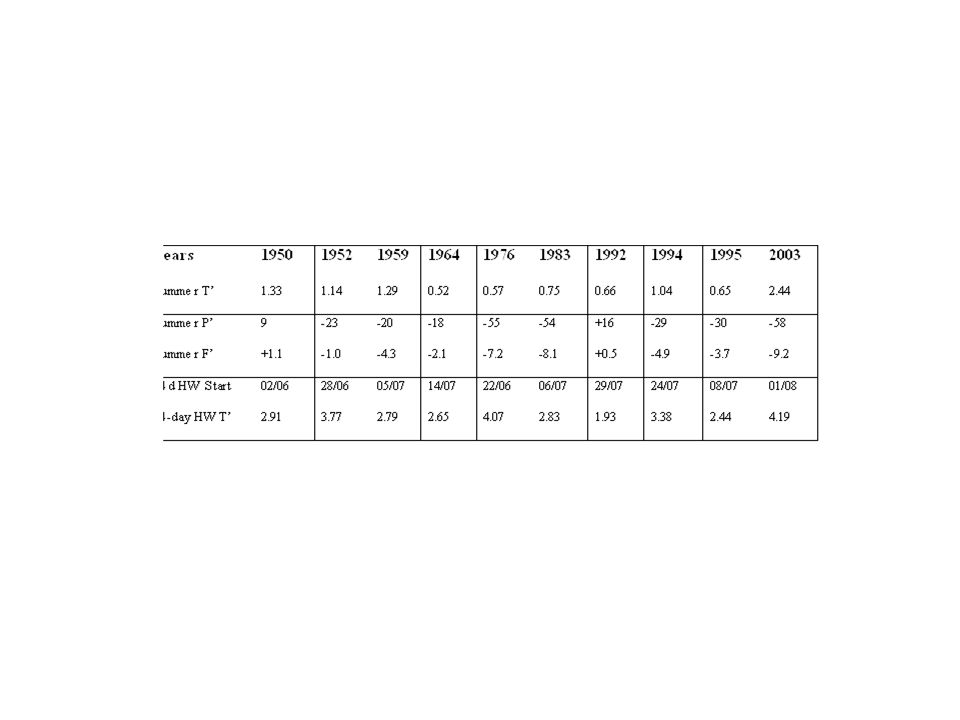
20. Figure 1: a) Summertime (JJA) anomaly composites (°C) over the hottest 10 summers in the 1948- 2004 period; b) same as a) but for JJA precipitation frequency (%). Stations where the anomaly is significant at the 90% level are marked by a black bullet; We will now check the anomaly decomposition on a 57 year dataset of station measurement in Europe for temperature and precipitation frequency. We select the 10 hottest years: Vautard et al 2007. GRL Hot summers: 1950 1952 1959 1964 1976 1983 1992 1994 1995 2003

21. c) Average anomalies, over the hottest 10 years, of maximal daily temperatures that would obtain by a sole change in the frequencies of summertime weather regimes [Cassou et al., 2005], as a function of the corresponding actual average anomalies. Each point corresponds to a station. See the methods section for details of calculation; d) Same as c) for precipitation frequencies. Reconstructed anomalies of Tmax and precipitation frequency. The reconstruction is always too cold and too wet. Temperature Precipitation

22. There is another mechanism that must be responsible for the strong temperature and precipitation anomalies. A good candidate: SOIL MOISTURE. Heatwaves have been observed to be preceeded by precipitation deficit (Huang and Van den Dool 1992 J. Clim. Figure 1: a) Summertime (JJA) anomaly composites (°C) over the hottest 10 summers in the 1948-2004 period; b) same as a) but for JJA precipitation frequency (%). Stations where the anomaly is significant at the 90% level are marked by a black bullet;

23. precipitation deficit Dry soil Less evapotranspiration Less latent Cooling. Less clouds Hot soil More sensible Heat flux Hot PBL Soil moisture controls the energy balance between the earth surface and the atmosphere by modulating sensible and latent (evaporation) heat fluxes.

24. Response of the UKMO GCM to prescribed values of soil moisture (Wet – Dry) Rowntree and Bolton (1983) TemperatureEvaporation Precipitation An old example

25. precipitation deficit Dry soil Less evapotranspiration Less latent Cooling. Less clouds Hot soil More sensible Heat flux Hot PBL Soil moisture controls the energy balance between the earth surface and the atmosphere by modulating sensible and latent (evaporation) heat fluxes. The Soil Moisture - Precipitation feedback High amplitude temperature and moisture variation are maintained by a feedback between soil moisture and precipitation (Schär et al 1999).

26. A more recent example from the group of Christophe Schär in Zurich Fischer et al 2007 - GRL

27. Fischer et al 2005 Regional GCM integrations of the year 2003, with prescribred soil moisture anomalies Control integrationsPerturbed integrations

28. Fischer et al 2005 Time evolution integrated over France

29. Mid-way summary Two ingredients for a good Heatwave: 1.A persistent anticyclonic regime 2.A dry soil moisture anomaly

30. Northward propagation of drought (Vautard et al 2007, GRL) Figure: a) Average rainfall frequency anomaly (% of days) (January–April) for the 10 years containing the hottest summers listed in Table 1 of the Auxiliary Material. The color scale is as in Figure 1b. The figures that would obtain for the winter only (January- march, not shown) or from January to May are rather similar to this one; b) Same as a) for averages of the month of May only; c) Same as a) for June; d) Difference between the early summer (June and July) maximal hot-summer temperature anomalies when southerly wind occurs at the station and that obtained for northerly wind. At each station, days are classified into 2 classes according to the sign of the mean daily surface meridional wind field. The 58- year average maximal temperature is calculated and subtracted from the hot- summer average to obtain mean anomalies. Then the difference between “southerly” and “northerly” mean anomalies is shown in panel d). The figure shows that temperature anomalies, in the 10 hottest summers, are higher in southerly wind conditions than in northerly wind conditions. e) As in d) for rainfall frequency (% of days). Stations where the differences are significant at the 90% level are marked with a black bullet.

31. Figure 3: Detrended summertime (JJA) daily maximum temperature anomalies, averaged over European stations, as a function of year (in black), together with the detrended anomaly of precipitation frequency averaged in the 42°N-46°N latitude band during preceding winter and early spring (January to May), in red. Temperature anomalies are in °C while precipitation frequencies anomalies are in %. In order to assess the sensitivity to the chosen latitude band for precipitation frequency, 2° northward and southward shifts are applied and results are also represented. Yellow bars indicate the years selected in the hottest 10 summer years. A predictor in the mediterranean region? Spring precipitation at different band of latitude and summer temperature Data from weather stations + a water budget model. Wilmott and Matsuura 2001.

33. Test of the drought propagation by mesoscale modeling (credit: Matteo Zampieri, LMD)

34. MM5 Integration details(credit: Matteo Zampieri, LMD) Simulations domain: most of Europe (excluding the Northern part of the Scandinavian peninsula) and a large part of the Atlantic Ocean. Forced by the ECMWF (ERA40) or NCAR-NCEP reanalyses with a 6-hour rate. Resolution: 36 km at the centre of the domain. 85x125 grid points and 23 vertical levels. MM5 3.7.3 model version Reisner microphysics, Kain-Fritsch convection scheme, MRF PBL scheme CCM2 radiation scheme. NOAH land-surface 4-layer scheme. twin simulation, starting on 1 June, for all the 10 hottest summers, differing only by their initial soil moisture south of 46N: 1)'wet' simulation. Initial volumetric soil moisture content of 30%. 2)'dry' simulation Initial volumetric soil moisture content of 15%. North of 46N initial soil moisture content is taken from the ERA40 ECMWF reanalysis data, when possible, or the NCAR-NCEP reanalysis data.

35. Temperature July Dry - WetJuly - June, Dry - Wet (80% run)

36. Precipitation July Dry - WetJuly - June, Dry - Wet

37. Soil moistureshort wave radiation

38. Sensible heat flux Latent heat flux

39. Mid-way summary Heat propagates northward from the mediterranean region: 1.By propagation of drought (over France) 2.By propagation of anomalous coudiness (over Germany)

40. Water balance on a layer of soil In a hot summer day, a mature tree can evaporate 2000 liters of water! …water for one week… At this point, we really need to study the dynamics of soil water, and its interaction with the atmosphere

41. PART 2 A simple model of the interaction of soil moisture and the atmospheric planetary boundary layer 1.Box model analysis of the feedback 2.1d (latitude) model Northward propagation 3.Effect of vegetation dynamics

42. PART 2 A simple model of the interaction of soil moisture and the atmospheric planetary boundary layer 1.Box model analysis of the feedback 2.1d (latitude) model Northward propagation 3.Effect of vegetation dynamics

43. Free troposphere Box model description (D’Andrea et al 2006 GRL) Planetary Boundary Layer Soil EP QsQs 1000 m 0.5 m Leakage divergence

44. Evaporation Rate (Laio et al 2001)

45. Evaporation Rate (can be used alternatively) Penman Monteith formula (FAO 56), modified and : resistence parameters (aerodynamic and bulk) Psychrometric constant (hPa per Kelvin )

46. Leakage Sensible heat flux Precipitation Rate and Runoff (1) (Laio et al 2001)

47. Convection Where: The above formulas for cooling and drying are obtained using the reduction of enthalpy and conserving relative humidity: Reminder:

48. Precipitation Rate and Runoff (2) Not all the water that is lifted in the free troposphere by convection precipitates. The fraction of precipitated water depends on the intensity of convection. f is 0.9 for strong convection and 0.25 for weak convection

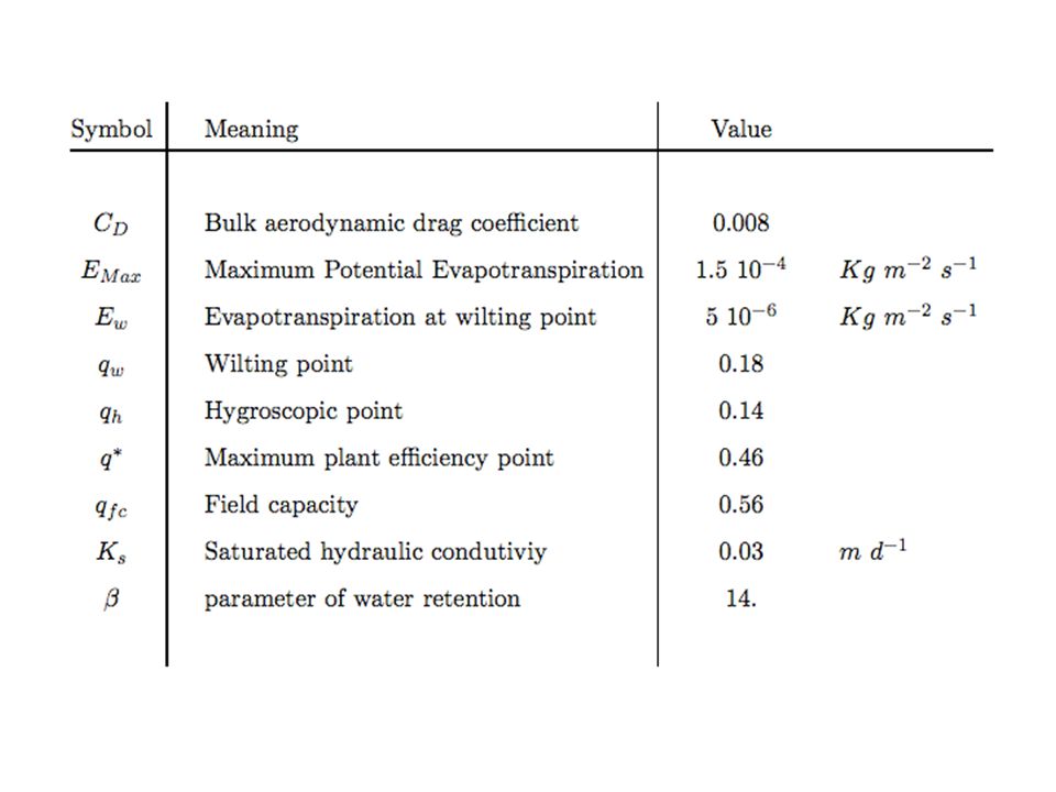
49. Equilibrium states As a function of initial soil moisture condition Some parameter values:

50. Hysteresis cycle obtained by varying Fq Air temperature Soil moisture Dependence on the large scale flux convergence

51. Stochastically forced integration Fq is perturbed stochastically every 5 days. Values varying between -1 and 3 mm/day. Flat distribution Cool and moist regime Dry and warm regime Observed data D’Odorico and Porporato 2003, PNAS

52. Two developments of the 0-d model: 1)1-d model: northward propagation 2)0-d model: dynamical vegetation

53. Free troposphere Box model description Planetary Boundary Layer Soil E0E0 P QsQs 1000 m 0.5 m Leakage divergence b ETET qsTsqsTs aqaaqa Baudena et al., 2007, in preparation MODEL DESCRIPTIONMODEL DESCRIPTION

54. Free troposphere Box model description Soil E0E0 P QsQs 1000 m 0.5 m Leakage divergence ETET MODEL DESCRIPTIONMODEL DESCRIPTION Baudena et al., 2007, in preparation

55. Wet/cool Dry/hot Wet/cool Dry/hot Initial conditions of vegetation cover b Initial conditions of soil moisture q s RESULTSRESULTS naturalnatural cultivatedcultivated Baudena et al., 2007, in preparation

56. vegetation cover b soil moisture q s RESULTSRESULTS Stochastic F q, “natural” vegetation Baudena et al., 2007, Glob Ch. Biol. Submitted

57. vegetation cover b soil moisture q s RESULTSRESULTS Stochastic F q, “cultivated” vegetation Baudena et al., 2007, Glob Ch. Biol., submitted

58. Results from 1-d model Equilibrium

59. Results from 1-d model DAY 1

60. Results from 1-d model DAY 30

61. Results from 1-d model DAY 60

62. Results from 1-d model DAY 90

63. Conclusions Two criteria are necessary for the occurrence of a heat and drought wave: 1.The establishment and presistence of an anticyclonic regime. 2. A condition of dry soil. When both criteria are met, the soil moisture - precipitation feedback can maintain large amplitudes of anomaly. Heat propagates northward from the Mediterranean region: 1.By propagation of drought (over France) 2.By propagation of anomalous cloudiness (over Germany) The initial content in soil water (and vegetation state) at the beginning of the summer is a crucial parameter. It is more likely that one summer is either in one or the other state and stay there, rather than a transition occur during the season (counterexample: summer 2006). Hypothesis: the dependence of precipitation efficiency on convection intensity can be at the base of the soil moisture - precipitation feedback. “Natural” vegetation increases the probability of the system of being in the wet/cool state as compared to “cultivated”.

64. Conclusions Differential E-P in a meridionally well mixed atmosphere can explain the northward propagation of the drought anomaly. (Still very sensitive to the model parameters. It depends strongly on the stability properties of the two regimes.)

65. Fig.: The visualization displays TERRA MODIS (MODerate resolution Imaging Spectroradiometer) derived land surface temperature data of 1km spatial resolution. The difference in land surface temperature is calculated by subtracting the average of all cloud free data during 2000, 2001, 2002 and 2004 from the ones in measured in 2003, covering the date range of July 20 - August 20. (Cite this image as: Image by Reto St-böckli, Robert Simmon and David Herring, NASA Earth Observatory, based on data from the MODIS land team. Correspondance: rstockli@climate.gsfc.nasa.gov). Thank you