1. Dr. Deshi Ye yedeshi@zju.edu.cn
Divide-and-conquer
Dr. Deshi Ye

2. Divide and Conquer 分治法 Divide:
the problem into a number of subproblems that are themselves smaller instances of the same type of problem.
Conquer:
Recursively solving these subproblems. If the subproblems are small enough, solve them straightforward.
Combine:
the solutions to the subproblems into
the solution of original problem.

3. Most common usage
Break up problem of size n into two equal parts of size n/2.
Solve two parts recursively
Combine two solutions into overall solution in linear time.

4. Which are more difficult?
Divided
Conquer
Combine

5. Sort Obviously application
Sort a list of names.
Organize an MP3 library.
Display Google PageRank results.
List RSS news items in reverse chronological order.
Problems become easy once items are in sorted order
Find the median.
Find the closest pair.
Binary search in a database.
Identify statistical outliers.
Find duplicates in a mailing list.

6. Non-obvious applications
Data compression.
Computer graphics.
Computational biology.
Supply chain management.
Book recommendations on Amazon.
Load balancing on a parallel computer.
....

7. Merge Sort John von Neumann 1945. If n = 1, done.
MERGE-SORT A[1 . . n]
If n = 1, done.
Recursively sort A[ n/2 ] and A[ n/2 n ] .
“Merge” the 2 sorted lists.
Divide
Conquer
Combine
Key subroutine: “Merge”

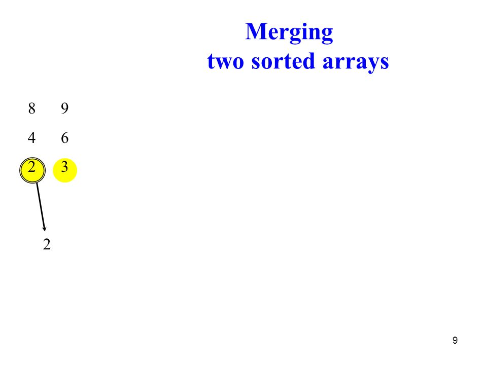
8. Merging two sorted arrays8 4 2 9 6 3

9. Merging two sorted arrays8 4 2 9 6 3 2

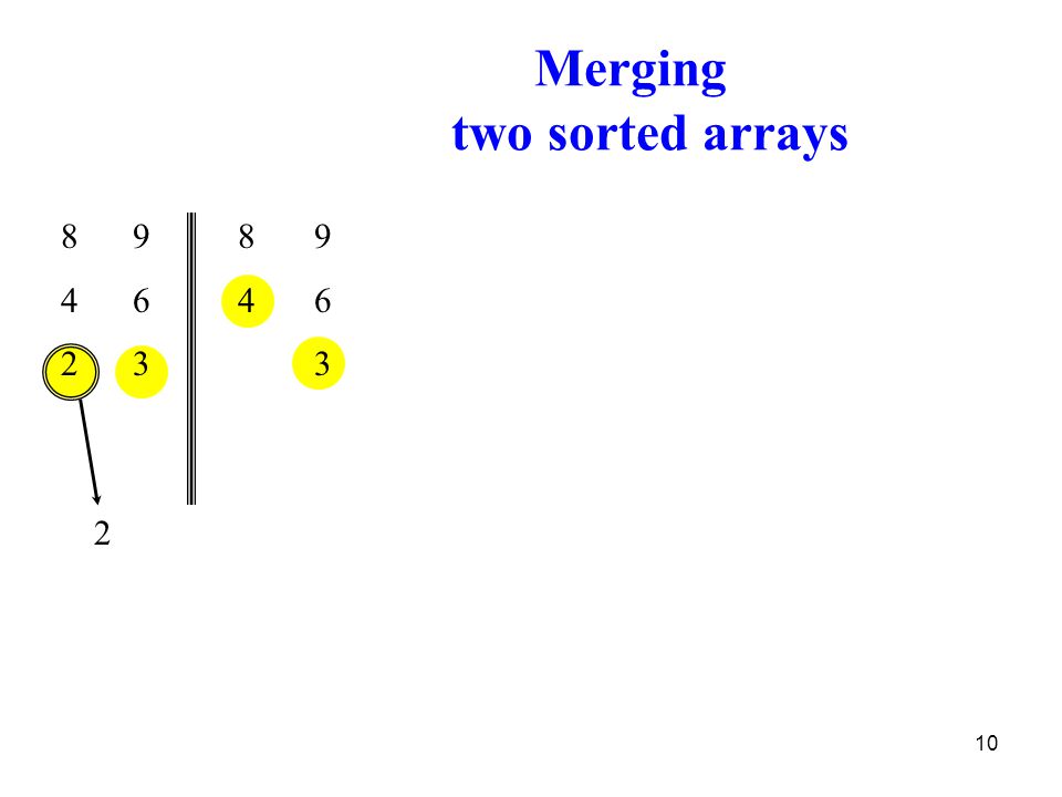
10. Merging two sorted arrays8 4 2 9 6 3 8 4 9 6 3 2

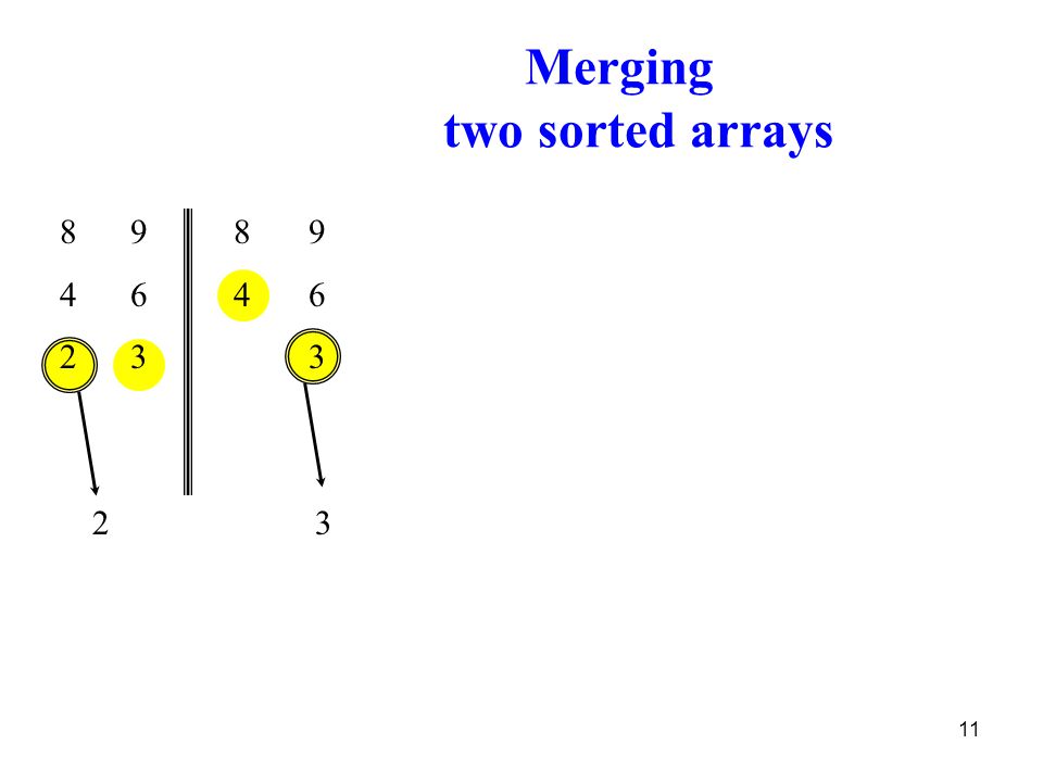
11. Merging two sorted arrays8 4 2 9 6 3 8 4 9 6 3 3 2

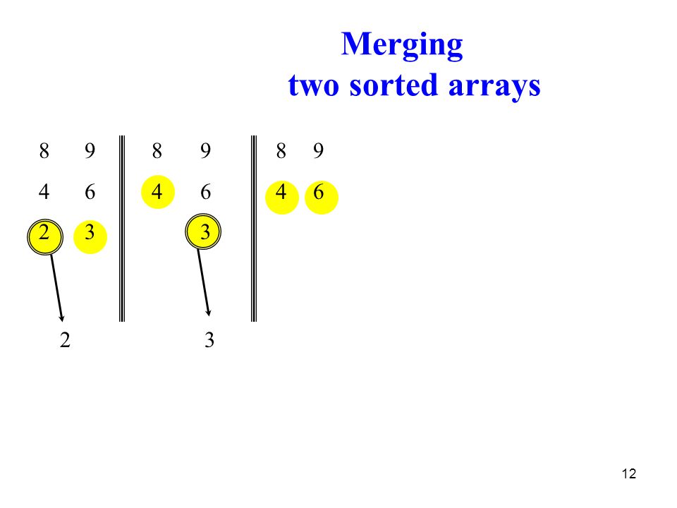
12. Merging two sorted arrays8 4 2 9 6 3 8 4 9 6 3 8 4 9 6 3 2

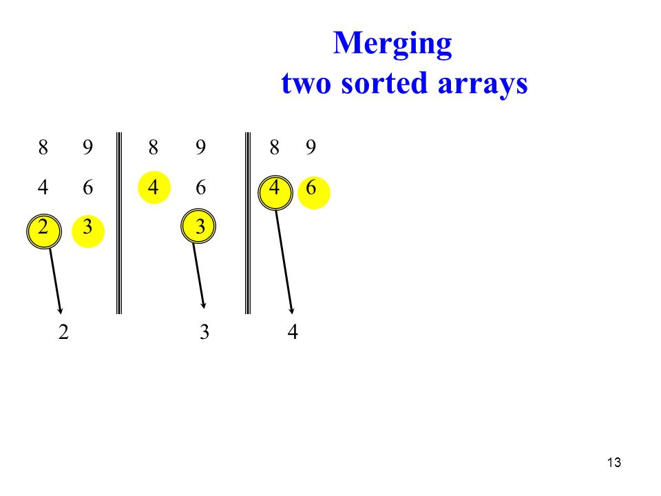
13. Merging two sorted arrays8 4 2 9 6 3 8 4 9 6 3 8 4 9 6 3 2 4

14. Merging two sorted arrays8 9 6 8 4 2 9 6 3 8 4 9 6 3 8 4 9 6 3 2 4

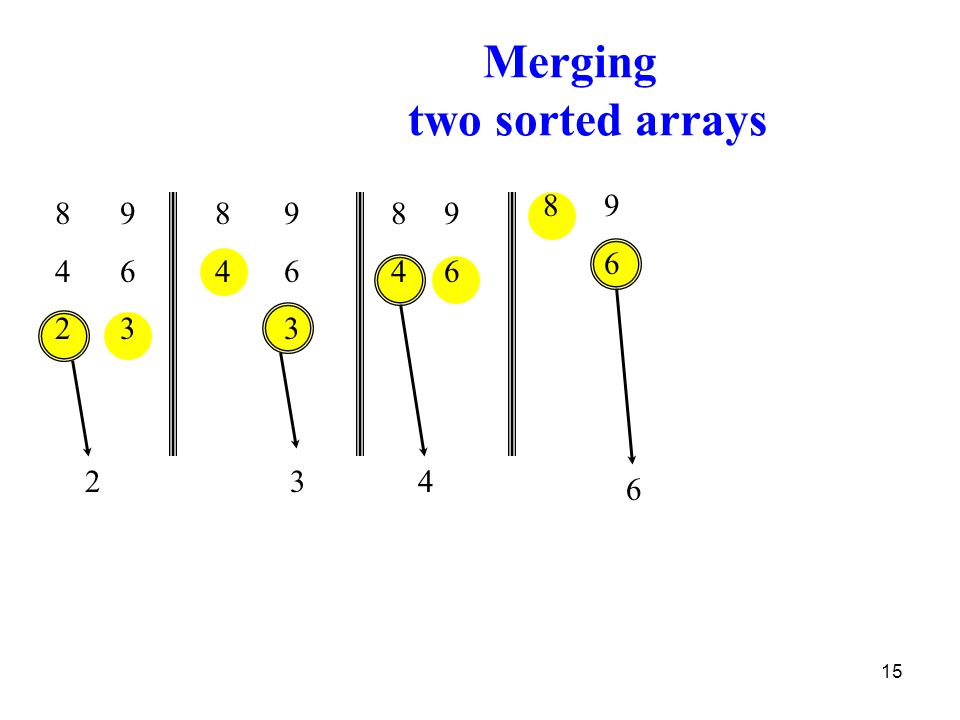
15. Merging two sorted arrays8 9 6 8 4 2 9 6 3 8 4 9 6 3 8 4 9 6 3 2 4 6

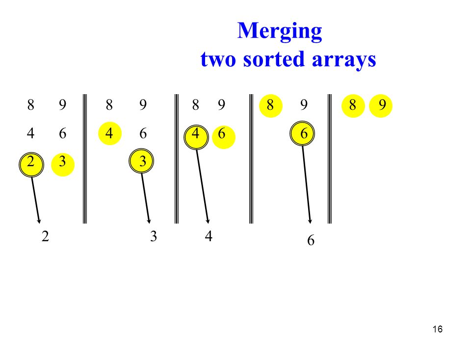
16. Merging two sorted arrays8 4 2 9 6 3 8 4 9 6 3 8 4 9 6 8 9 6 8 9 2 3 4 6

17. Merging two sorted arrays8 4 2 9 6 3 8 4 9 6 3 8 4 9 6 8 9 6 8 9 2 3 4 6 8

18. Merging two sorted arrays8 4 2 9 6 3 8 4 9 6 3 8 4 9 6 8 9 6 8 9 2 3 4 6 8 9
Time = Q(n) to merge a total of n elements (linear time).

19. Analyzing merge sort MERGE-SORT A[1 . . n] T(n) Q(1) 2T(n/2)
Q(n)
MERGE-SORT A[1 . . n]
If n = 1, done.
Recursively sort A[ n/2 ] and A[ n/2 n ] .
“Merge” the 2 sorted lists
Sloppiness: Should be T( n/2 ) + T( n/2 ) , but it turns out not to matter asymptotically.

20. Recurrence for merge sort
T(n) =
Q(1) if n = 1;
2T(n/2) + Q(n) if n > 1.
We shall usually omit stating the base case when T(n) = Q(1) for sufficiently small n, but only when it has no effect on the asymptotic solution to the recurrence.
Master theorem can find a good upper bound on T(n).

21. Recursion tree
Solve T(n) = 2T(n/2) + cn, where c > 0 is constant.

22. Recursion tree Solve T(n) = 2T(n/2) + cn, where c > 0 is constant.

23. Recursion tree Solve T(n) = 2T(n/2) + cn, where c > 0 is constant.

24. Recursion tree Solve T(n) = 2T(n/2) + cn, where c > 0 is constant.

25. Recursion tree Solve T(n) = 2T(n/2) + cn, where c > 0 is constant.…
Q(1)

26. Recursion tree Solve T(n) = 2T(n/2) + cn, where c > 0 is constant.
h = lg n
cn/4
cn/4
cn/4
cn/4 …
Q(1)

27. Recursion tree Solve T(n) = 2T(n/2) + cn, where c > 0 is constant.
h = lg n
cn/4
cn/4
cn/4
cn/4 …
Q(1)

28. Recursion tree Solve T(n) = 2T(n/2) + cn, where c > 0 is constant.
h = lg n
cn/4
cn/4
cn/4
cn/4 …
Q(1)

29. Recursion tree Solve T(n) = 2T(n/2) + cn, where c > 0 is constant.
h = lg n
cn/4
cn/4
cn/4
cn/4 cn … …
Q(1)

30. Recursion tree Solve T(n) = 2T(n/2) + cn, where c > 0 is constant.
h = lg n
cn/4
cn/4
cn/4
cn/4 cn … …
Q(1)
#leaves = n
Q(n)

31. Recursion tree Solve T(n) = 2T(n/2) + cn, where c > 0 is constant.
h = lg n
cn/4
cn/4
cn/4
cn/4 cn … …
Q(1)
#leaves = n
Q(n)
Total = Q(n lg n)

32. Computing For any integer x and n, please compute the value
Calculate the Fibonacci number
Hint:

33. Integer Multiplication

34. Integer Multiplication
Complex multiplication.
(a + bi) (c + di) = x + yi.
Grade-school.
x = ac - bd, y = bc + ad.
Gauss
x = ac - bd, y = (a + b) (c + d) - ac - bd.
Remark.
Improvement if no hardware multiply.
4 multiplications, 2 additions
3 multiplications,
5 additions

35. Integer Arithmetic
Add. Given two n-bit integers a and b, compute a + b.
Grade-school. Θ(n) bit operations.
Multiply. Given two n-bit integers a and b, compute a * b.
Grade-school. Θ(n2) bit operations.

36. To multiply two n-bit integers
Multiply four n/2-bit integers.
Add two n/2-bit integers, and shift to obtain result.
x = (10ma +b), y = (10mc +d)
Ex: x = , m=5, a=12345, b=67890
(10ma +b) (10mc +d) = 102mac + 10m(bc +ad)+ bd

37. Multiply (x, y, n):
If n = 1
return x y
Else
m = n/2
a = x/10m, b = x mod 10m;
c = y/10m, d= y mod 10m
e = multiply(a, c,m)
f = multiply(b, d, m)
g = multiply(b, c, m)
h = multiply(a, d, m)
Reutrn 102m e + 10m(g+h) +f

38. Ac+ bd - (a - b)(c - d) = bc + ad
Fast multiply
T(n) = 4T(n/2) + O(n), T(1) = 1
Which solves to T(n) = O(n2) by the master theorem.
Anatolii, Karatsuba in 1962:
T(n) = 3 T(n/2) + O(n)
T(n) = O(nlg3)=O(n1.585)
Ac+ bd - (a - b)(c - d) = bc + ad

39. FastMultiply (x, y, n):
If n = 1
return x y
Else
m = n/2
a = x/10m, b = x mod 10m;
c = y/10m, d= y mod 10m
e = multiply(a, c,m)
f = multiply(b, d, m)
g = multiply(a - b, c - d, m)
Reutrn 102m e + 10m(e+ f - g) +f

40. Fast Integer Division Too
Integer division. Given two n-bit (or less) integers a and b, compute quotient
q = a / b and remainder r = a mod b.
Complexity of integer division is same as multiplication. To compute quotient q:
Approximate x = 1 / b using Newton's method
xi+1 = 2xi – bxi2 apply fast multiply
After log n iterations, q = [a x]

41. Newton Method
Goal. Given a function f (x), find a value x* such that f(x*) = 0.
Newton's method.
Start with initial guess x0.
Compute a sequence
of approximations:

42. Exam.
Approximately compute x = 1 / t using exact arithmetic. Let t = 7. t =
x0 = 0.1
x1 = 0.13
x2 =
x3 =
x4 =
x5 =
x6 =

43. Newton’s method xn+1 = xn – f(xn)/f′(xn)
Let x = 1/b, f(x) = 1/x – b, f′ (x)= - 1/x2

44. Integer Division: Newton's Method
(q, r) = NewtonDivision(s, t)
Choose x to be unique fractional power of 2 in interval (1 / (2t), 1 / t ]
repeat lg n times
x = 2x – t x2
set q = integer(s x )
set r = s – q t

45. Analysis Lemma 1. Iterates converge monotonically.
Lemma 2. Iterates converge quadratically to 1 / t:

46. Root
The approximation of
Let f(x) = x2 - a

47. Matrix multiplication
Given two n-by-n matrices X and Y, compute Z = XY. j i * = Y Z X

48. Running time
Brute force:
Fundamental question: can you improve?

49. Matrix multiplication
Divide-and-conquer
Divide: partition A and B into n/2-by-n/2 blocks.
Conquer: multiply 8 n/2-by-n/2 recursively.
Combine: add appropriate products using 4 matrix additions.

50. Runnig time

51. Key Idea
Key idea. multiply 2-by-2 block matrices with only 7 multiplications.
where

53. Fast Matrix multiply Fast matrix multiplication. [Strassen, 1969]
Divide: partition X and Y into n/2-by-n/2 blocks.
Compute: 14 n/2-by-n/2 matrices via 10 matrix additions.
Conquer: multiply 7 pairs of n/2-by-n/2 matrices recursively.
Combine: 7 products into 4 terms using 8 matrix additions.
Analysis

54. Fast Matrix Multiplication in Theory
Q: Multiply two 2-by-2 matrices with 7 scalar multiplications?
A: Yes! [Strassen, 1969]
Q: Multiply two 2-by-2 matrices with 6 scalar multiplications?
A: Impossible. [Hopcroft and Kerr, 1971]
Q: Two 3-by-3 matrices with 21 scalar multiplications?
A: Also impossible.
New: Can be solved in 23 scalar multiplications. [Laderman, 1976; Courtois 2011]

55. Fast Matrix Multiplication in Practice
Implementation issues.
Sparsity.
Caching effects.
Numerical stability.
Odd matrix dimensions.
Crossover to classical algorithm around n = 128.
Common misperception: “Strassen is only a theoretical curiosity.”
Advanced Computation Group at Apple Computer reports 8x speedup on G4 Velocity Engine when n =2,500.
Range of instances where it's useful is a subject of controversy.

56. Fast Matrix Multiplication in Theory
Best known. O(n2.376)
[Coppersmith-Winograd, 1987]
Conjecture.
Caveat. Theoretical improvements to Strassen are progressively less practical.

57. Fast Fourier Transform
Applications:
Optics, acoustics, quantum physics, telecommunications, radar, control systems, signal processing, speech recognition, data compression, image processing, seismology, mass spectrometry…
Digital media. [DVD, JPEG, MP3, H.264]
Medical diagnostics. [MRI, CT, PET scans, ultrasound]
Numerical solutions to Poisson's equation.
Shor's quantum factoring algorithm

58. The FFT is one of the truly great computational developments of [the 20th] century. It has changed the face of science and engineering so much that it is not an exaggeration to say that life as we know it would be very different without the FFT.
-- Charles van Loan

59. Polynomials: Coefficient Representation
Polynomial. [coefficient representation]
Add. O(n) arithmetic operations.
Multiply (convolve). O(n2) using brute force.

60. Polynomials: Point-Value Representation
[Gauss, PhD thesis] A degree n polynomial is uniquely characterized by its values at any n+1 distinct points. (Two points determine a line)
y=A(xi ) xi

61. Polynomials: Point-Value Representation
Polynomial. [point-value representation]
Add. O(n) arithmetic operations.
Multiply (convolve). O(n) but need 2n-1 points.

62. Evaluate How to evaluate A(x0) for the point (x0,y0) Horner’s Rule:
It takes for computing all A(x0)

63. Converting Between Two Representations: Brute Force
Coefficient point-value. Given a polynomial A(xi) , evaluate at n different point xi, i.e. to compute
Hence, we could get (xi, yi)

64. Converting Between Two Representations: Brute Force
point-value Coefficient. Given n distinct points and n values
find unique polynomial
Vander-monder matrix is invertible

65. Vander-monde Matrix Vander-monde matrix is invertible iff xi different
Matrix , its determinant is

66. Converting Between Two Polynomial Representations
Tradeoff. Fast evaluation or fast multiplication. We want both!
Goal. Make all ops fast by efficiently converting between two representations.
Representation
Multiply
Evaluate
Coefficient
O(n2)
O(n)
Point value

67. Algorithm: Polynomial multiplication
Input.
Coefficient of two polynomials, A and B of degree n
Output.
Their product C=AB
Selection.
Pick some points x0 , ..., x2n-2
Evaluation
Compute A(xi), B(xi)
Multiplication.
Ci = A(xi)B(xi)
Interpolation.
Recover coefficient of C
O(n2)
O(n)
O(n2)

68. Coefficient representation
Polynomial multiply
Coefficient representation
a0 ,a1 ,...,an-1
b0 ,b1 ,...,bn-1
c0 ,c1 ,...,c2n-2
Inverse FFT O(n log n)
FFT O(n log n)
Point-value multiply
A(x0) ... A(x2n-2)
B(x0) ... B(x2n-2)
Point-value
representation
C(x0)...C(x2n-2)
O(n)

69. Coefficient to Point-Value: Intuition
Divide. Break polynomial up into even and odd powers.
Intuition. Choose two points to be

70. T(n) = 2T(n/2) + O(n), hence T(n)= O(n lgn) Question left:
Can evaluate polynomial of degree n at 2 points by evaluating two polynomials of degree n/2 at 1 point.
T(n) = 2T(n/2) + O(n), hence T(n)= O(n lgn)
Question left: +1 -1 +1 -1 +1 -1

71. Discrete Fourier Transform
Key idea. Choose where is principal nth root of unity.
Fourier Matrix
Discrete Fourier transform

72. Roots of Unity
Def. An nth root of unity is a complex number x such that xn = 1.
Fact. The nth root of unity are:
where and
Proof. b r a

73. Root of unity
Fact. The (n/2)th roots of unity are:
Note.

74. Fast Fourier Transform
Goal. Evaluate a degree n-1 polynomial
At its nth root of unity
Divide.

75. FFT con.
Conquer. Evaluate Aeven(x) and Aodd(x) at its (n/2)th root of unity:
Combine.

76. FFT Summary
Theorem. FFT algorithm evaluates a degree n-1 polynomial at each of the nth roots of unity in O(n log n) steps.
Running time.
Now, coefficient -> point-value is done

77. Point - coefficient
To get the coefficient from point value representation

78. Inverse FFT
Claim. Inverse of Fourier matrix is given by following formula.
Consequence. To compute inverse FFT, apply same algorithm but use as nth root of unity

79. Inverse FFT: Proof of Correctness
Claim. Fn and Gn are inverses.
Pf.
Summation lemma.
Pf. If k is a multiple of n,
is a root of
otherwise , we have

80. Inverse FFT summary
Theorem. Inverse FFT algorithm evaluates a degree n-1 polynomial at each of the nth roots of unity in O(n log n) steps.
Running time

81. Coefficient representation
Polynomial multiply
Theorem. Can multiply two degree n-1 polynomials in O(n log n) steps.
Coefficient representation
a0 ,a1 ,...,an-1
b0 ,b1 ,...,bn-1
c0 ,c1 ,...,c2n-2
Inverse FFT O(n log n)
FFT O(n log n)
Point-value multiply
A(x0) ... A(x2n-2)
B(x0) ... B(x2n-2)
Point-value
representation
C(x0)...C(x2n-2)
O(n)

82. Big Num Class java.math.BigNum Number representation:
Using radix b positional notation, an interger N
Can be written as
b >1 is the base
For all i, ni are the digits of N written in base b
Class java.math.BigNum

83. Some big numbers
Pi:

84. e