1. Divide-and-Conquer
CIS 606
Spring 2010

2. Analyzing Divide-and-Conquer Algorithms
Use a recurrence to characterize the running time of a divide-and-conquer algorithm.
Solving the recurrence gives us the asymptotic running time.
A recurrence is a function is defined in terms of
one or more base cases, and !
itself, with smaller arguments.

3. Analyzing Divide-and-Conquer Algorithms
Examples

4. Analyzing Divide-and-Conquer Algorithms
Many technical issues:
Floors and ceilings
Exact vs. asymptotic functions
Boundary conditions
In algorithm analysis, we usually express both the recurrence and its solution using asymptotic notation.
Example: T(n) = 2T(n/2) + Θ(n) with solution T(n) = Θ(n lg n).

5. Analyzing Divide-and-Conquer Algorithms
The boundary conditions are usually expressed as “T(n) = O(1) for sufficiently small n.”
When we desire an exact, rather than an asymptotic, solution, we need to deal with boundary conditions.
In practice, we just use asymptotics most of the time, and we ignore boundary conditions.

6. Maximum-Subarray Problem
Input: An array A[1..n] of numbers.
Output: Indices i and j such that A[i..j] has the greatest sum of any nonempty, contiguous subarray of A, along with the sum of the values in A[i..j].
Scenario
You have the prices that a stock traded at over a period of n consecutive days.
When should you have bought the stock? When should you have sold the stock?
Even though it’s in retrospect, you can yell at your stockbroker for not recommending these buy and sell dates.

7. Maximum-Subarray Problem
To convert to a maximum-subarray problem, let A[i] = (price after day i ) - (price after day (i -1)).
Then the nonempty, contiguous subarray with the greatest sum brackets the days that you should have held the stock.
If the maximum subarray is A[i..j], then should have bought just before day i (i.e., just after day i - 1) and sold just after day j .
Why do we need to find the maximum subarray? Why not just “buy low, sell high”?

8. Maximum-Subarray Problem
Lowest price might occur after the highest price.
But wouldn’t the optimal strategy involve buying at the lowest price or selling at the highest price?
Not necessarily:
Maximum profit is $3 per share, from buying after day 2 and selling after day 3.
Yet lowest price occurs after day 4 and highest occurs after day 1.

9. Maximum-Subarray Problem
Can solve by brute force: check all Θ(n2) subarrays.
Can organize the computation so that each subarray A[i..j] takes O(1) time, given that you’ve computed A[i..j – 1], so that the brute-force solution takes Θ(n2) time.
Solving by divide-and-conquer
Use divide-and-conquer to solve in O(n lg n) time.
Subproblem: Find a maximum subarray of A[low..high].
In original call, low = 1, high = n.

10. Solving by divide-and-conquer
Divide the subarray into two subarrays of as equal size as possible. Find the midpoint mid of the subarrays, and consider the subarrays A[low..mid] and A[mid + 1..high].
Conquer by finding maximum subarrays of A[low..mid] and A[mid + 1..high].
Combine by finding a maximum subarray that crosses the midpoint, and using the best solution out of the three (the subarray crossing the midpoint and the two solutions found in the conquer step).
This strategy works because any subarray must either lie entirely on one side of the midpoint or cross the midpoint.

11. Solving by divide-and-conquer
Finding the maximum subarray that crosses the midpoint
Not a smaller instance of the original problem: has the added restriction that the subarray must cross the midpoint.
Again, could use brute force. If size of A[low..mid] is n, would have n/2 choices for left endpoint and n/2 choices for right endpoint, so would have Θ(n2) combinations altogether.
Can solve in linear time.

12. Solving by divide-and-conquer
Any subarray crossing the midpoint A[mid] is made of two subarrays A[i..mid] and A[mid j], where low ≤ i ≤ mid and mid < j ≤ high.
Find maximum subarrays of the form A[i..mid] and A[mid j] and then combine them.
Procedure to take array A and indices low, mid, high and return a tuple giving indices of maximum subarray that crosses the midpoint, along with the sum in this maximum subarray:

13. Solving by divide-and-conquer

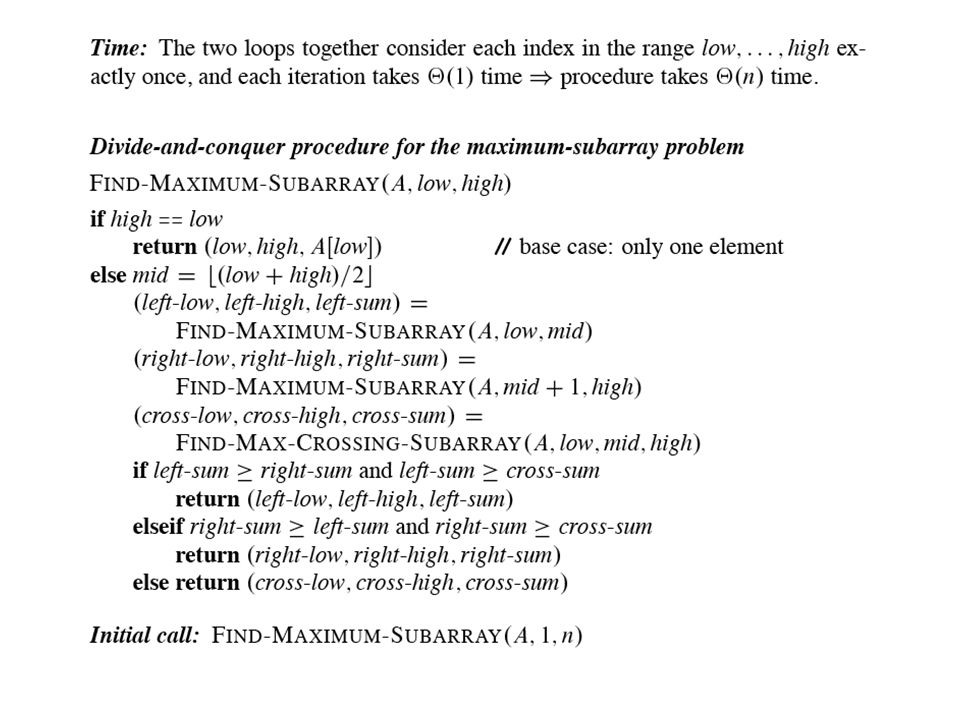
15. Solving by divide-and-conquer
Divide by computing mid.
Conquer by the two recursive calls to FIND-MAXIMUM-SUBARRAY.
Combine by calling FIND-MAX-CROSSING-SUBARRAY and then determining which of the three results gives the maximum sum.
Base case is when the subarray has only 1 element.

16. Analysis
Simplifying assumption: Original problem size is a power of 2, so that all subproblem sizes are integer.
Let T(n) denote the running time of FIND-MAXIMUM-SUBARRAY on a subarray of n elements.
Base case: Occurs when high equals low, so that n = 1. The procedure just returns ⇒ T(n) = Θ(1).

17. Analysis Recursive case: Occurs when n > 1.
Dividing takes Θ(1) time.
Conquering solves two subproblems, each on a subarray of n / 2 elements. Takes T(n/2) time for each subproblem ⇒ 2T(n/2) time for conquering.
Combining consists of calling FIND-MAX-CROSSING-SUBARRAY, which takes Θ(n) time, and a constant number of constant-time tests ⇒Θ(n) + Θ(1) time for combining.

18. Analysis

19. Strassen’s method for matrix multiplication

20. Strassen’s method for matrix multiplication

21. Strassen’s method for matrix multiplication
Is Θ(n3) the best we can do? Can we multiply matrices in o(n3)?
Seems like any algorithm to multiply matrices must take Ω(n3) time:
Must compute n2 entries
Each entry is the sum of n terms
But with Strassen’s method we can multiply in o(n3)
Strassen’s method runs in Θ(nlg 7) time.
2.80 ≤ lg 7 ≤ 2.81
Hence, runs in Θ(n2.81) time

22. Simple divide-and-conquer method
As with the other divide-and-conquer algorithms, assume that n is a power of 2.
Partition each of A;B;C into four n/2 × n/2 matrices:
Rewrite C = A ⋅B as

23. Simple divide-and-conquer method
giving the four equations
Each of these equations multiplies two n/2 × n/2 matrices and then adds their n/2 × n/2 products.
Use these equations to get a divide-and-conquer algorithm

24. Simple divide-and-conquer method

25. Matrix Multiplication
Analysis
Let T(n) be the time to multiply two n/2 × n/2 matrices.
Best case: n = 1. Perform one scalar multiplication: Θ(1).
Recursive case: n > 1.
Dividing takes Θ(1) time using index calculations.
Conquering makes 8 recursive calls, each multiplying two n/2 × n/2 matrices ⇒ 8T(n/2).
Combining takes Θ(n2) time to add n/2 × n/2 matrices 4 times.

26. Matrix Multiplication
Recurrence is
Can use master method to show that it has solution T(n) = Θ(n3). Asymptotically, no better than the obvious method.

27. Matrix Multiplication
When setting up recurrences, can absorb constant factors into asymptotic notation, but cannot absorb a constant number of subproblems.
Although we absorb the 4 additions of n/2 × n/2 matrices into the Θ(n2) time we cannot lose the 8 in front of the T(n/2) term.
If we absorb the constant number of subproblems, then the recursion tree would not be “bushy” and would instead just be a linear chain.

28. Strassen’s Method
Idea: Make the recursion tree less bushy. Perform only 7 recursive multiplications of n/2 × n/2 matrices, rather than 8. Will cost several additions of n/2 × n/2 matrices, but just a constant number more ⇒ can still absorb the constant factor for matrix additions into the Θ(n2) term.

29. Strassen’s Method Algorithm
As in the recursive method, partition each of the matrices into four n/2 × n/2 submatrices. Time: Θ(1).
Create 10 matrices S1, S2,…, S10. Each is n/2 × n/2 and is the sum or difference of two matrices created in previous step. Time: Θ(n2) to create all 10 matrices.
Recursively compute 7 matrix products P1, P2,…, P10 each n/2 × n/2.
Compute n/2 × n/2 submatrices of C by adding and subtracting various combinations of the Pi. Time: Θ(n2).

30. Strassen’s Method Analysis: Recurrence will be
By the master method, solution is T(n) = Θ(nlg 7).

31. Details Step 2, create the 10 matrices
Add or subtract n/2 × n/2 matrices 10 times ⇒ time is Θ(n / 2).

32. Details Step 3, create the 7 matrices
The only multiplications needed are in the middle column; right-hand column just shows the products in terms of the original submatrices of A and B.

33. Details Step 4, Add and subtract the Pi to construct submatrices of C:
To see how these computations work, expand each right-hand side, replacing each Pi with the submatrices of A and B that form it, and cancel terms:

34. Details

35. Theoretical and practical notes
Strassen’s algorithm was the first to beat Θ(n3) time, but it’s not the asymptotically fastest known. A method by Coppersmith and Winograd runs in O(n2.376) time.
Practical issues against Strassen’s algorithm:
Higher constant factor than the obvious Θ(n3)-time method.
Not good for sparse matrices.
Not numerically stable: larger errors accumulate than in the obvious method.
Submatrices consume space, especially if copying.
Crossover point somewhere between n = 8 and 400.

36. Substitution method Guess the solution.
Use induction to find the constants and show that the solution works.
Example

37. Substitution method Guess: T(n) = n lg n + n. Induction:
Basis: n =1 ⇒ n lg n + n = 1 = T(n)
Inductive step: Inductive hypothesis is that T(k) = k lg k + k for all k < n. We’ll use this inductive hypothesis for T(n / 2).

38. Substitution method Generally, we use asymptotic notation:
We would write T(n) = 2T(n / 2) + Θ(n).
We assume T(n) = O(1) for sufficiently small n.
We express the solution by asymptotic notation: T(n) = Θ(n lg n).
We don’t worry about boundary cases, nor do we show base cases in the substitution proof.
T(n) is always constant for any constant n.
Since we are ultimately interested in an asymptotic solution to a recurrence, it will always be possible to choose base cases that work.
When we want an asymptotic solution to a recurrence, we don’t worry about the base cases in our proofs.
! When we want an exact solution, then we have to deal with base cases.

39. Substitution method For the substitution method: Example
Name the constant in the additive term.
Show the upper (O) and lower (Ω) bounds separately. Might need to use different constants for each.
Example
T(n) = 2 T(n / 2) + Θ(n). If we want to show an upper bound of T(n) = 2 T(n / 2) + Θ(n), we write T(n) ≤ 2 T(n / 2) + cn for some positive constant c.

40. Substitution method Upper bound:
Guess: T(n) ≤ d n lg n for some positive constant d. We are given c in the recurrence, and we get to choose d as any positive constant. It’s OK for d to depend on c.

41. Substitution method
Lower bound: Write T(n) ≥ 2 T(n / 2) + cn for some positive constant c.
Guess: T(n) ≥ d n lg n for some positive constant d.
Therefore, T(n) = θ(n lg n)

42. Substitution method

43. Substitution method

44. Recursion trees
Use to generate a guess. Then verify by substitution method.
Example:

45. Recursion trees
There are log3n full levels, and after log3/2n levels, the problem size is down to 1.
Each level contributes ≤ c n.
Lower bound guess: ≥ d n log3n = Ω(n lg n) for some positive constant d.
Upper bound guess: ≤ d n log3/2n = O(n lg n) for some positive constant d.
Then prove by substitution.

46. Recursion trees
Upper bound:

47. Recursion trees
Lower bound:

48. Master method Used for many divide-and-conquer recurrences of the form
T(n) = aT(n/b) + f(n), where a ≥ 1, b > 1, f(n) > 0.
Based on the master theorem (Theorem 4.1).

49. Master method

50. Master method

51. Master method