Download presentation
Presentation is loading. Please wait.

1
Development of Simulation Methodologies for Forced Mixers Anastasios Lyrintzis School of Aeronautics & Astronautics Purdue University

2
Acknowledgements Indiana 21 st Century Research and Technology Fund Prof. Gregory Blaisdell Rolls-Royce, Indianapolis (W. Dalton, Shaym Neerarambam) L. Garrison, C. Wright, A. Uzun, P-T. Lew
 L. Garrison, C. Wright, A. Uzun, P-T. Lew.")
3
Motivation Airport noise regulations are becoming stricter. Jet exhaust noise is a major component of aircraft engine noise Lobe mixer geometry has an effect on the jet noise that needs to be investigated.

4
Methodology 3-D Large Eddy Simulation for Jet Aeroacoustics RANS for Forced Mixers Coupling between LES and RANS solutions (Semi-empirical method)
")
5
3-D Large Eddy Simulation for Jet Aeroacoustics

6
Objective Development and full validation of a Computational Aeroacoustics (CAA) methodology for jet noise prediction using: A 3-D Large Eddy Simulation (LES) code working on generalized curvilinear grids that provides time-accurate unsteady flow field data A surface integral acoustics method using LES data for far-field noise computations
 methodology for jet noise prediction using: A 3-D Large Eddy Simulation (LES) code working on generalized curvilinear grids that provides time-accurate unsteady flow field data A surface integral acoustics method using LES data for far-field noise computations")
8
Numerical Methods for LES 3-D Navier-Stokes equations 6 th -order accurate compact differencing scheme for spatial derivatives 6 th -order spatial filtering for eliminating instabilities from unresolved scales and mesh non-uniformities 4 th -order Runge-Kutta time integration Localized dynamic Smagorinsky subgrid-scale (SGS) model for unresolved scales
 model for unresolved scales")
10
Computational Jet Noise Research Some of the biggest jet noise computations: Freund’s DNS for Re D = 3600, Mach 0.9 cold jet using 25.6 million grid points (1999) Bogey and Bailly’s LES for Re D = 400,000, Mach 0.9 isothermal jets using 12.5 and 16.6 million grid points (2002, 2003) We studied a Mach 0.9 turbulent isothermal round jet at a Reynolds number of 100,000 12 million grid points used in our LES
 Bogey and Bailly’s LES for Re D = 400,000, Mach 0.9 isothermal jets using 12.5 and 16.6 million grid points (2002, 2003) We studied a Mach 0.9 turbulent isothermal round jet at a Reynolds number of 100, million grid points used in our LES")
11
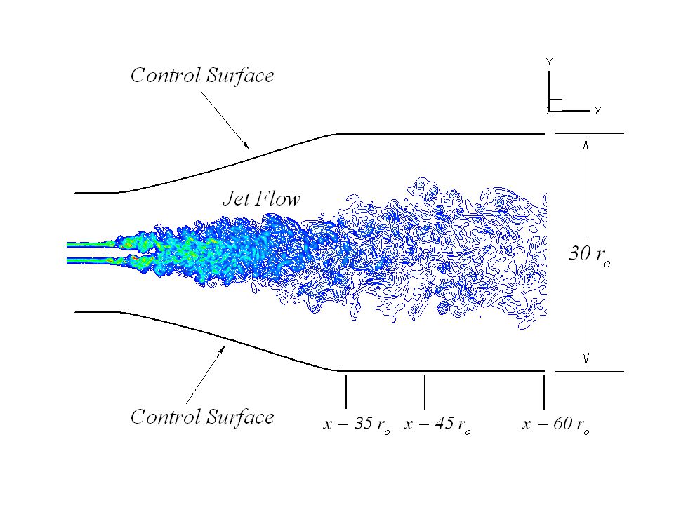
Computation Details Physical domain length of 60r o in streamwise direction Domain width and height are 40r o 470x160x160 (12 million) grid points Coarsest grid resolution: 170 times the local Kolmogorov length scale One month of run time on an IBM-SP using 160 processors to run 170,000 time steps Can do the same simulation on the Compaq Alphaserver Cluster at Pittsburgh Supercomputing Center in 10 days
 grid points Coarsest grid resolution: 170 times the local Kolmogorov length scale One month of run time on an IBM-SP using 160 processors to run 170,000 time steps Can do the same simulation on the Compaq Alphaserver Cluster at Pittsburgh Supercomputing Center in 10 days")
16
Mean Flow Results Our mean flow results are compared with: Experiments of Zaman for initially compressible jets (1998) Experiment of Hussein et al. (1994) Incompressible round jet at Re D = 95,500 Experiment of Panchapakesan et al. (1993) Incompressible round jet at Re D = 11,000
 Incompressible round jet at Re D = 95,500 Experiment of Panchapakesan et al. (1993) Incompressible round jet at Re D = 11,000.")
24
Jet Aeroacoustics Noise sources located at the end of potential core Far field noise is estimated by coupling near field LES data with the Ffowcs Williams–Hawkings (FWH) method Overall sound pressure level values are computed along an arc located at 60r o from the jet nozzle Cut-off Strouhal number based on grid resolution is around 1.0
 method Overall sound pressure level values are computed along an arc located at 60r o from the jet nozzle Cut-off Strouhal number based on grid resolution is around 1.0")
27
OASPL results are compared with: Experiment of Mollo-Christensen et al. (1964) Mach 0.9 round jet at Re D = 540,000 (cold jet) Experiment of Lush (1971) Mach 0.88 round jet at Re D = 500,000 (cold jet) Experiment of Stromberg et al. (1980) Mach 0.9 round jet at Re D =3,600 (cold jet) SAE ARP 876C database Jet Aeroacoustics (continued)
 Mach 0.9 round jet at Re D = 540,000 (cold jet) Experiment of Lush (1971) Mach 0.88 round jet at Re D = 500,000 (cold jet) Experiment of Stromberg et al. (1980) Mach 0.9 round jet at Re D =3,600 (cold jet) SAE ARP 876C database Jet Aeroacoustics (continued).")
31
Conclusions Localized dynamic SGS model stable and robust for the jet flows we are studying Very good comparison of mean flow results with experiments Aeroacoustics results are encouraging Valuable evidence towards the full validation of our CAA methodology has been obtained

32
Near Future Work Simulate Bogey and Bailly’s Re D = 400,000 jet test case using 16 million grid points 100,000 time steps to run About 150 hours of run time on the Pittsburgh cluster using 200 processors Compare results with those of Bogey and Bailly to fully validate CAA methodology Do a more detailed study of surface integral acoustics methods

34
Can a realistic LES be done for Re D = 1,000,000 ? Assuming 50 million grid points provide sufficient resolution: 200,000 time steps to run 30 days of computing time on the Pittsburgh cluster using 256 processors Only 3 days on a near-future computer that is 10 times faster than the Pittsburgh cluster

35
Future Work Extend methodology to handle: –Noise from unresolved scales –Supersonic flow –Solid boundaries (lips) –Complicated (mixer) geometries multi-block code
 –Complicated (mixer) geometries multi-block code")
36
RANS for Forced Mixers

37
Objective Use RANS to study flow characteristics of various flow shapes

38
What is a Lobe Mixer?

39
Internally Forced Mixed Jet Bypass Flow Mixer Core Flow Nozzle Tail Cone Exhaust Flow Exhaust / Ambient Mixing Layer Lobed Mixer Mixing Layer

40
Forced Mixer H Lobe Penetration (Lobe Height) H:
 H:")
41
3-D Mesh

42
WIND Code options 2 nd order upwind scheme 1.7 million/7 million grid points 8-16 zones 8-16 LINUX processors Spalart-Allmaras/ SST turbulence model Wall functions

43
Grid Dependence Density Contours 1.7 million grid points Density Contours 7 million grid points

44
Grid Dependence 1.7 million grid points7 million grid points Density Vorticity Magnitude

45
Spalart-Allmaras and Menter SST Turbulence Models Spalart-Allmaras Menter SST

46
Spalart-Allmaras and and Menter SST at Nozzle Exit Plane Spalart SST Density Vorticity Magnitude

47
Mean Axial Velocity at x = 2.88” (High Penetration) ¼ Scale Spalart at x = 2.88/4” experiment Spalart Allmaras
 ¼ Scale Spalart at x = 2.88/4 experiment Spalart Allmaras")
48
Mean Axial Velocity at x = 2.88” (High Penetration) ¼ Scale Menter SST at x = 2.88/4” experiment Menter SST
 ¼ Scale Menter SST at x = 2.88/4 experiment Menter SST")
49
Spalart-Allmaras vs. Menter SST The Spalart-Allmaras model appears to be less dissipative. The vortex structure is sharper and the vorticity magnitude is higher at the nozzle exit. The Menter SST model appears to match experiments better, but the experimental grid is rather coarse and some of the finer flow structure may have been effectively filtered out. Still unclear which model is superior. No need to make a firm decision until several additional geometries are obtained.

50
Geometry at Mixer Exit Low PenetrationMid PenetrationHigh Penetration

51
DENSITY CONTOURS (¼ Scale) Low Penetration Mid Penetration
 Low Penetration Mid Penetration")
52
Vorticity Magnitude at Nozzle Exit (¼ Scale Geometry) Low Penetration Mid Penetration High Penetration
 Low Penetration Mid Penetration High Penetration")
53
Turbulent Kinetic Energy at Nozzle Exit (¼ Scale Geometry) Low PenetrationMid Penetration High Penetration
 Low PenetrationMid Penetration High Penetration")
54
Preliminary Conclusions 1.7 million grid is adequate Further work is needed comparing the turbulence models and results for different penetration lengths

55
Future Work Analyze the flow fields and compare to experimental acoustic and flow-field data for additional mixer geometries. Further compare the two turbulence models. If possible, develop qualitative relationship between mean flow characteristics and acoustic performance.

56
Implementing RANS Inflow Boundary Conditions for 3-D LES Jet Aeroacoustics

57
Objectives Implement RANS solution and onto 3-D LES inflow BCs as initial conditions. Investigate the effect of RANS inflow conditions on: –Reynolds Stresses –Far-field sound generated

58
Implementation Method RANS grid too fine for LES grid to match. Since RANS grid has high resolution, linear interpolation will be used. LES RANS

59
Issues and Challenges Accurate resolution of outgoing vortex with LES grid. Accurate resolution of shear layer near nozzle lip. May need to use an intermediate Reynolds number eg. Re = 400,000

60
Final Conclusion Methodologies (LES, RANS, coupling) are being developed to study noise from forced mixers
 are being developed to study noise from forced mixers")
Similar presentations


 Lyrintzis Ph.D. Aerospace Engineering, Cornell University (1988) –Helicopter blade-vortex interactions.>")


>")


