1. Chapter 15 Above: GPS time series from southern California after removing several curve fits to the data

2. Fitting curves to data is very common in Earth sciences Has applications in virtually all subdiscipline Two things to keep in mind: Data is noisy Data is discrete (non-continuous) Curve fitting can help overcome these issues (to some degree) Empirical Modeling: A type of modeling that involves fitting a curve to data and then using the equation of the curve to predict values From Wells & Coppersmith (1994) Extrapolations of Future Global Warming, IPCC (2007)

3. MATLAB provides several built-in functions to fit curves Many require the “Curve Fitting Toolbox”, or other toolboxes. We will only use the basic curve fitting functions that are part of standard MATLAB We will focus on polyfit, polyval, corrcoef, roots polyfit Fits data with a polynomial curve of a user-specified degree

4. Polynomials come in different orders or degrees 0 th order: a single constant value Examples: y = 4 y = 2.75 y = -12.1 1 st order: a linear equation (independent var is to 1 st power) Examples: y = 4x y = 3.2x + 7 y = -8.2x – 21.3 2 nd order: a quadratic equation Examples: y = 5x 2 y = 2.9x 2 + 7 y = -1.8x 2 – 7.4x + 1.4 3 rd order: a cubic equation Examples: y = 7x 3 y = 4.6x 3 + 2 y = 2.4x 3 + 3.5x 2 + 3.2x + 7.3 n th order: a polynomial where “n” is the largest exponent Can be represented as a row vector in MATLAB Interpreted by “polyval” as coefficients of a polynomial

5. Using polyval requires a lot less typing Saves time!

6. A first order polynomial is a linear equation

7. Roots of a function: Where function = 0 Useful in sciences because we often want to know where parameters return to zero Also useful for finding min/max of data and equations 1 st order polynomial: 1 root 2 nd order polynomial: 0, 1, or 2 roots 3 rd order polynomial: up to 3 roots n th order polynomial: up to n roots Warning! Some polynomials have no real roots, but do have roots with imaginary numbers Recall, the discriminant b 2 – 4ac

8. This means that… Discriminant > 0 Polynomial

9. This means that… Has no real roots! Discriminant < 0 Polynomial

10. This means that… Has 4 real roots! Polynomial

11. Polynomials are easy to deal with in MATLAB As the order of the polynomial increases… So does the complexity of the curve Remember the Taylor Series? You can fit any function with an infinite series of polynomials More polynomials = better fit Polyfit is similar except it fits a single polynomial to data

12. A Simple Test… Fit 5 collinear points with linear equation

13. Use polyfit to perform a least squares fit of a 1 st order polynomial i.e. a linear fit

14. While there are better ways to evaluate goodness of fit… It is beyond our scope to cover all methods for goodness of fit Take a Stats course! Correlation coefficient, R, is one commonly used measure R 2 = tells the % of your data’s variance that is explained by a linear fit R 2 = 0.95 means 95% of your data variance is explained by linear fit. What is good enough? Depends on the situation

15. Make synthetic data with noise See if fit is reasonable

17. Increasing the order of the polynomial allows for more complex curves to be fit Be careful to not over-fit your data! MATLAB will give a warning if the result is poorly conditioned

20. What if data is unevenly spaced? How could you estimate an evenly spaced data set? Interpolate it Interpolation: The process of estimating values in between data points What if data is limited in range? How could you estimate data beyond your data range? Extrapolate values Very prone to errors. Should always be done with extreme caution Extrapolation: The process of estimating values beyond the bounds of your data MATLAB provides several ways to interpolate data I will only cover using “interp1” and “polyfit”

21. You can use a best fit curve to interpolate Make sure the curve fits data well Best fit curves tend to smooth data Will not honor your collected data points! This is why formal interpolation is typically preferred Be careful about extrapolating!

22. interp1: interpolates 1D data See also interp2 and interp3 for 2D/3D interp1 has several options Read the documentation We will only use linear or spline methods

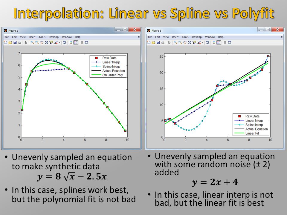
23. Linear Interpolation Resultant data is boxy Min/Max will not exceed the original data Interpolation using splines Resultant data has smooth curves Min/Max may exceed the original data Both methods honor y-vals at original data

25. “interp1” can be used to extrapolate beyond input data limits Use ‘extrap’ option interp1(x,y,’linear’,’extrap’) Use with great caution! Use with great caution! Extrapolation is highly prone to errors Extrapolation should only be a last resort Which method worked best? None! Extrapolation is a bad idea If you have to do it, only go very slightly beyond your data limits

26. MATLAB offers several built-in functions for curve fitting and resampling data We covered only polyfit and interp1 There is no way to know a priori which method is most appropriate for your data Take statistics classes Always test your curve fits Know what relationship to expect between data (if possible) Polynomial fits are not appropriate for all data sets May want to explore other methods E.g. Fourier Analysis / Spectral Analysis MATLAB has TONS of other curve fitting and resampling options in various toolboxes Don’t use toolbox commands this class, but feel free to explore them in your research