1. Basic Properties of signal, Fourier Expansion and it’s Applications in Digital Image processing. Md. Al Mehedi Hasan Assistant Professor Dept. of Computer Science & Engineering RUET, Rajshahi-6204. E-mail: mehedi_ru@yahoo.com

2. Signals Signal is defined by its Amplitude, Frequency and Phase Signals can be analog or digital. Analog signals can have an infinite number of values in a range. Digital signals can have only a limited number of values.

3. Comparison of analog and digital signals

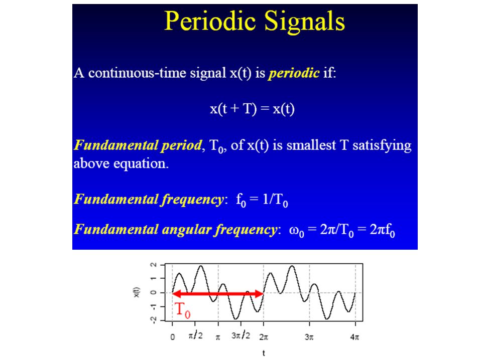
4. Periodic Signal Both analog and digital signals can be of two forms: Periodic and Aperiod. A signal is a periodic if it completes a pattern within a measurable time frame, called a period, and repeats that pattern over identical subsequent period.

5. Periodic signals can be classified as simple or composite. Periodic signals (continue) simple composite

7. Aperiodic Signal An aperiodic, or nonperiodic, signal has no patterns.

8. Amplitude The Amplitude of a signal is the value of the signal at any point on the wave.

9. Period and Frequency Period refers to the amount of time, a signal needs to complete one cycle. Frequency refers to the number of periods in one second. Frequency and period are the inverse of each other.

10. 3.10 Units of period and frequency

11. Phase The term phase describes the position of the waveform relative to time zero.

12. Two signals with the same phase and frequency, but different amplitudes

13. 3.13 Two signals with the same amplitude and phase, but different frequencies

14. 3.14 Three sine waves with the same amplitude and frequency, but different phases

15. 3.15 The power we use at home has a frequency of 60 Hz. The period of this sine wave can be determined as follows: Example

16. 3.16 The period of a signal is 100 ms. What is its frequency in kilohertz? Example Solution First we change 100 ms to seconds, and then we calculate the frequency from the period (1 Hz = 10 −3 kHz).

17. 3.17 If a signal does not change at all, its frequency is zero. If a signal changes instantaneously, its frequency is infinite. Note

18. 3.18 A sine wave is offset 1/6 cycle with respect to time 0. What is its phase in degrees and radians? Example Solution We know that 1 complete cycle is 360°. Therefore, 1/6 cycle is

19. Sine and Cosine Functions Periodic functions General form of sine and cosine functions:

20. Sine and Cosine Functions Special case: A=1, b=0, α=1 π

21. Sine and Cosine Functions (cont’d) Cosine is a shifted sine function: Shifting or translating the sine function by a const b

22. Sine and Cosine Functions (cont’d) Changing the amplitude A

23. Sine and Cosine Functions (cont’d) Changing the period T=2π/|α| e.g., y=cos(αt) period 2π/4=π/2 shorter period higher frequency (i.e., oscillates faster) α =4 Frequency is defined as f=1/T Different notation: sin(αt)=sin(2πt/T)=sin(2πft)

24. Definition of Radian One radian is the measure of a central angle that intercepts an arc equal in length to the radius of the circle. See Figure. Algebraically, this means that where θ is measured in radians.

28. Why Radian Measure? In most applications of trigonometry, angles are measured in degrees. In more advances work in mathematics, radian measure of angles is preferred. Radian measure allows us to treat the trigonometric functions as functions with domains of real numbers, rather than angles.

29. Linear speed measures how fast the particle moves, and angular speed measures how fast the angle changes.

32. Frequency is a metric for expressing the rate of oscillation in a wave. For planar and longitudinal waves, this often expressed in oscillations-per-second or Hz. Angular frequency used for expressing rates of rotation, similar to revolutions-per-second, and is usually expressed in radians-per-second. It can be thought of as a wave with a constant amplitude where the amplitude rotates in a circle in space. Frequency and Angular Frequency

33. Different Notation of Sine and Cosine Functions Changing the period T=2π/|α| e.g., y=cos(αt) period 2π/4=π/2 shorter period higher frequency (i.e., oscillates faster) α =4 Frequency is defined as f=1/T

34. Different Notation of Sine and Cosine Functions (continue) Fundamental Frequency?

35. Time Domain and Frequency Domain Time Domain: The time-domain plot shows changes in signal amplitude with respect to time. Phase and frequency are not explicitly measure on a time-domain plot. Frequency Domain: The time-domain plot shows changes in signal amplitude with respect to frequency.

36. 3.36 The time-domain and frequency-domain plots of a sine wave

37. 3.37 The time domain and frequency domain of three sine waves

38. Frequency Spectrum and Bandwidth The frequency spectrum of a signal is the combination of all sine wave signals that make up that signal. The bandwidth of a signal is the width of the frequency spectrum.

39. Jean Baptiste Joseph Fourier Fourier was born in Auxerre, France in 1768 – Most famous for his work “La Théorie Analitique de la Chaleur” published in 1822 – Translated into English in 1878: “The Analytic Theory of Heat” Nobody paid much attention when the work was first published One of the most important mathematical theories in modern engineering

40. The Big Idea = Any function that periodically repeats itself can be expressed as a sum of sines and cosines of different frequencies each multiplied by a different coefficient – a Fourier series Images taken from Gonzalez & Woods, Digital Image Processing (2002)

41. 3.41 Fourier analysis A single-frequency sine wave is not useful in some situation We need to use a composite signal, a signal made of many simple sine waves. According to Fourier analysis, any composite signal is a combination of simple sine waves with different frequencies, amplitudes, and phases.

42. 3.42 Composite Signals and Periodicity If the composite signal is periodic, the decomposition gives a series of signals with discrete frequencies. If the composite signal is nonperiodic, the decomposition gives a combination of sine waves with continuous frequencies.

43. Fourier Series of composite periodic signal Every composite periodic signal can be represented with a series of sine and cosine functions. The functions are integral harmonics of the fundamental frequency “f” of the composite signal. Using the series we can decompose any periodic signal into its harmonics.

44. 3.44 A composite periodic signal

45. 3.45 Decomposition of a composite periodic signal in the time and frequency domains

46. The time and frequency domains of a nonperiodic signal Nonperiodic signal

47. Fourier Series

48. Where Fourier Series

49. Meaning of Coefficients

50. An equation with many faces There are several different ways to write the Fourier series.

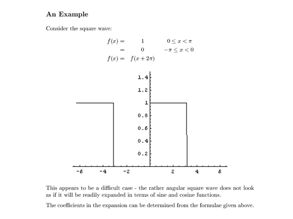
55. Examples of Signals and the Fourier Series Representation

56. Sawtooth Signal

57. Application

58. When we deal with a one dimensional signal (time series), it is quite easy to understand what the concept of frequency is. Frequency is the number of occurrences of a repeating event per unit time. For example, in the figure below, we have 3 cosine functions with increasing frequencies cos(t), cos(2t), and cos(3t). Spatial Frequency in image

59. Spatial Frequency in image (con..)

60. So, we know that a sequence of such numbers gives us the feeling that cos(t) is a low frequency signal. How we can create an image of these numbers? Let scale the numbers to the range 0 and 255: Considering that values are intensity values, we can obtain the following image. Spatial Frequency in image (con..)

61. This is our first image with a low frequency component. We have a smooth transition from white to black and black to white. However, it is still difficult to say anything since we have not seen an image with high frequency. If we repeat all the steps for cos(3t), we obtain the following image: where we have sudden jumps to black. You can try the same experiment for different cosines. By looking at two examples, we can say that if there are sharp intensity changes in an image, those regions correspond to high frequency components. On the other hand, regions with smooth transitions correspond to low frequency components. Spatial Frequency in image (con..)

62. We now have an idea for one dimensional image. It is time to switch to two dimensional representation of a signal. Let us first define a kind of two dimensional signal: f(x, y)=cos(kx) cos(ky). For example, the signal for k=1, we have: f(x, y)=cos(x) cos(y). Spatial Frequency in image (con..)

63. If you wonder, you can assign different k values (e.g. f(x,y)=cos(x)cos(3y) ) for the base cosine functions, and plot the result. Our goal is to create an image containing a single frequency component as much as possible. Let us pick a cosine signal with a low frequency: cos(t). Our corresponding two dimensional function will be f(x, y)=cos(x) cos(y). How we will obtain a two dimensional image from this function? This is the question! We are going to define a matrix and store the values of f(x,y) for different (x, y) pairs. Basically, we divide the angle range 0-2∏ into M=512 and N=512 regions for x and y, respectively. Spatial Frequency in image (con..)

64. Here are images for different k values. Values of k represents the level of frequency (from low to high) for k=0,….,20. Spatial Frequency in image (con..)

66. Similar to the 1D case, we can say that if the intensity values in an image changes dramatically, that image has high frequency components. Spatial Frequency in image (con..)

67. Frequency Domain In Images  Spatial frequency of an image refers to the rate at which the pixel intensities change  In picture on right: High frequences: Near center Low frequences: Corners

68. The Discrete Fourier Transform (DFT) 2-D case The Discrete Fourier Transform of f(x, y), for x = 0, 1, 2… M -1 and y = 0,1,2… N -1, denoted by F(u, v), is given by the equation: for u = 0, 1, 2… M -1 and v = 0, 1, 2… N -1.

69. The Inverse DFT It is really important to note that the Fourier transform is completely reversible. The inverse DFT is given by: for x = 0, 1, 2… M -1 and y = 0, 1, 2… N -1

70. Discrete Fourier transform (2-D)

71. The DFT and Image Processing Images taken from Gonzalez & Woods, Digital Image Processing (2002)

73. How con we connect broken text ?

74. How can we remove blemishes in a photograph?

75. How can we get the enhanced image from the original image? Enhanced image

76. Some Basic Frequency Domain Filters Images taken from Gonzalez & Woods, Digital Image Processing (2002) Low Pass Filter High Pass Filter

77. Smoothing Frequency Domain Filters Smoothing is achieved in the frequency domain by dropping out the high frequency components The basic model for filtering is: G(u,v) = H(u,v)F(u,v) where F(u,v) is the Fourier transform of the image being filtered and H(u,v) is the filter transform function Low pass filters – only pass the low frequencies, drop the high ones

78. Ideal Low Pass Filter Simply cut off all high frequency components that are a specified distance D 0 from the origin of the transform changing the distance changes the behaviour of the filter Images taken from Gonzalez & Woods, Digital Image Processing (2002)

79. Ideal Low Pass Filter (cont…) The transfer function for the ideal low pass filter can be given as: where D(u,v) is given as:

80. Ideal Low Pass Filter (cont…) Above we show an image, it’s Fourier spectrum and a series of ideal low pass filters of radius 5, 15, 30, 80 and 230 superimposed on top of it Images taken from Gonzalez & Woods, Digital Image Processing (2002)

81. Ideal Low Pass Filter (cont…) Images taken from Gonzalez & Woods, Digital Image Processing (2002) Original image Result of filtering with ideal low pass filter of radius 5 Result of filtering with ideal low pass filter of radius 30 Result of filtering with ideal low pass filter of radius 230 Result of filtering with ideal low pass filter of radius 80 Result of filtering with ideal low pass filter of radius 15

82. Lowpass Filtering Examples A low pass Gaussian filter is used to connect broken text Images taken from Gonzalez & Woods, Digital Image Processing (2002)

83. Lowpass Filtering Examples (cont…) Different lowpass Gaussian filters used to remove blemishes in a photograph Images taken from Gonzalez & Woods, Digital Image Processing (2002)

84. Thank You