Download presentation
Presentation is loading. Please wait.

1
Introduction to Statistics: Political Science (Class 6) Interactions Between Variables
 Interactions Between Variables")
2
Remember what regression “does” Identifies the coefficients that minimize the sum of the squared residuals For example…

3
DV: Obama Favorability Coef.SETP Strong Republican-1.6520.161-10.2900.000 Weak Republican-0.7040.197-3.5800.000 Lean Republican-1.2290.181-6.7900.000 Lean Democrat0.6540.1953.3400.001 Weak Democrat0.4570.1872.4400.015 Strong Democrat0.5790.1583.6500.000 Gender (female=1)0.0720.0870.8300.405 Age-0.0410.019-2.1400.033 Age 2 0.0440.0182.4300.015 Constant3.7840.5097.4300.000 These coefficients are the values that get us to the predicted values that minimize the sum of squared residuals
 Age Age Constant These coefficients are the values that get us to the predicted values that minimize the sum of squared residuals")
4
How? Simple formula for calculating coefficients in bivariate case. Not simple in multivariate case. In practice, MV analysis relies on matrix algebra. In theory, this can be done computationally by searching though every iteration of coefficient values.

5
We have covered Regression using: –Linear variables –Dichotomous indicators –Squared and logarithmic terms Today: what if the relationship between a predictor and outcome “depends”?

6
It depends! The effect ofondepends on Campaign ads……support for a candidate …whether a person watches TV. Number of missiles fired… …number of targets destroyed… …quality of targeting systems. GDP……life expectancy……whether the nation is democratic. ???

7
Regression models thus far Life Expectancy = β 0 + β 1 GDP + β 2 Democracy + u How do we interpret β 1 ? What if we expect the relationship between GDP and life expectancy to be different in democracies?

8
First, the mechanics Interaction term: one variable x another –E.g., Democracy x GDP We add this new variable to our model: –β 0 + β 1 GDP + β 2 Democracy + β 3 Democracy*GDP + u We’ll focus on countries with GDP per capita of $1000 or less in 1970 (most countries)
")
9
And viola! OK. What the heck does this mean? Coef.SETP GDP per capita0.0370.0049.8000.000 Democracy (1=yes)6.7092.4122.7800.007 Democracy*GDP-0.0130.006-2.1300.036 Constant41.4931.27032.6600.000
 Democracy*GDP Constant")
10
How many different predictor characteristics are we dealing with for each unit of analysis (country)? Coef.SETP GDP per capita0.0370.0049.8000.000 Democracy (1=yes)6.7092.4122.7800.007 Democracy*GDP-0.0130.006-2.1300.036 Constant41.4931.27032.6600.000 41.493 +.037*GDP + 6.709*Democracy – 0.013*Democracy*GDP + u Let’s start by crunching some numbers…
 Democracy*GDP Constant *GDP *Democracy – 0.013*Democracy*GDP + u Let’s start by crunching some numbers….")
11
41.493 + 0.037*GDP + 6.709*Democracy – 0.013*Democracy*GDP + u GDPDemocracy GDP (β) Democracy (β) Democracy x GDP (β)Constant Predicted Value Coefficients 0.0376.709-0.01341.493 000.0000041.493 25009.2000041.49350.693 500018.3990041.49359.892 750027.5990041.49369.092 1000036.7980041.49378.291 First for non-democracies (Democracy = 0)… Difference in predicted value (GDP=0 v. 1000) = 36.798
 =")
12
41.493 + 0.037*GDP + 6.709*Democracy – 0.013*Democracy*GDP + u Now for democracies (Democracy = 1)… GDPDemocracy GDP (β) Democracy (β) Democracy x GDP (β)Constant Predicted Value Coefficients 0.0376.709-0.01341.493- 010.0006.709041.49348.202 25019.2006.709-3.129741.49354.272 500118.3996.709-6.259441.49360.342 750127.5996.709-9.389141.49366.412 1000136.7986.709-12.518841.49372.482 Difference in predicted value (GDP=0 v. 1000) = 24.280
 =")
14
The slope on GDP per capita depends on the value of democracy It is 0.037 - 0.013*Democracy –So when democracy = 0, the coefficient (slope) on GDP is 0.037 –When democracy = 1, the coefficient is 0.037 – 0.013 (or 0.024) 41.493 + 0.037*GDP + 6.709*Democracy – 0.013*Democracy*GDP + u
 on GDP is –When democracy = 1, the coefficient is – (or 0.024) *GDP *Democracy – 0.013*Democracy*GDP + u")
15
This work symmetrically – i.e., the coefficient on Democracy also depends on the value of GDP –Specifically the estimated effect of being a democracy rather than not is 6.709-0.013*(GDP) Is one “side of the coin” better? 41.493 + 0.037*GDP + 6.709*Democracy – 0.013*Democracy*GDP + u

16
Never ever, ever… Coef.SETP GDP per capita0.0370.0049.8000.000 Democracy (1=yes)6.7092.4122.7800.007 Democracy*GDP-0.0130.006-2.1300.036 Constant41.4931.27032.6600.000 …interpret the coefficient on one of the components of an interaction without respect to the value of the other variable used in the interaction “components” of an interaction In some cases they might not even make sense!
 Democracy*GDP Constant …interpret the coefficient on one of the components of an interaction without respect to the value of the other variable used in the interaction components of an interaction In some cases they might not even make sense!")
17
Coef.SETP GDP per capita0.0370.0049.8000.000 Democracy (1=yes)6.7092.4122.7800.007 Democracy*GDP-0.0130.006-2.1300.036 Constant41.4931.27032.6600.000 So how do we interpret the statistical significance of a coefficient on an interaction? What does it mean to say this coefficient is statistically different from zero? The slope on GDP when Democracy=0 is significantly different from the slope when Democracy=1 (or, symmetrically, the slope on Democracy depends on the value of GDP…)
.")
18
We can also look at the coefficient on the interaction term and say… Coef.SETP GDP per capita0.0370.0049.8000.000 Democracy (1=yes)6.7092.4122.7800.007 Democracy*GDP-0.0130.006-2.1300.036 Constant41.4931.27032.6600.000 For every one unit increase in Democracy we expect the slope of the relationship between GDP and Life Expectancy to decrease by 0.013 OR, symmetrically… For every one unit increase in GDP we expect the slope of the relationship between Democracy and Life Expectancy to decrease by 0.013 Expected effect of Democracy when GDP per capita is 100?
 Democracy*GDP Constant For every one unit increase in Democracy we expect the slope of the relationship between GDP and Life Expectancy to decrease by OR, symmetrically… For every one unit increase in GDP we expect the slope of the relationship between Democracy and Life Expectancy to decrease by Expected effect of Democracy when GDP per capita is 100")
19
Support for Comparative Effectiveness Research For many medical conditions, doctors use different kinds of treatments, and there is no scientific agreement on which is best. For example, a patient may be experiencing a particular type of pain and it is unclear whether the best treatment is a drug, physical therapy, or surgery. Recently there has been discussion about the need for more research to determine which treatments are most effective for which patients. This is sometimes called comparative effectiveness research. Would you support or oppose government funding of research on the effectiveness of different medical treatments? Strongly Oppose (0) to Strongly Support (100)
 to Strongly Support (100).")
20
Party affiliation What would you expect about the relationship between party affiliation and support for CER? Coef.SETP Party Affiliation (-3=strong R; 3=strong D)4.5300.25617.6700.000 Constant59.9740.547109.7000.000
 Constant")
21
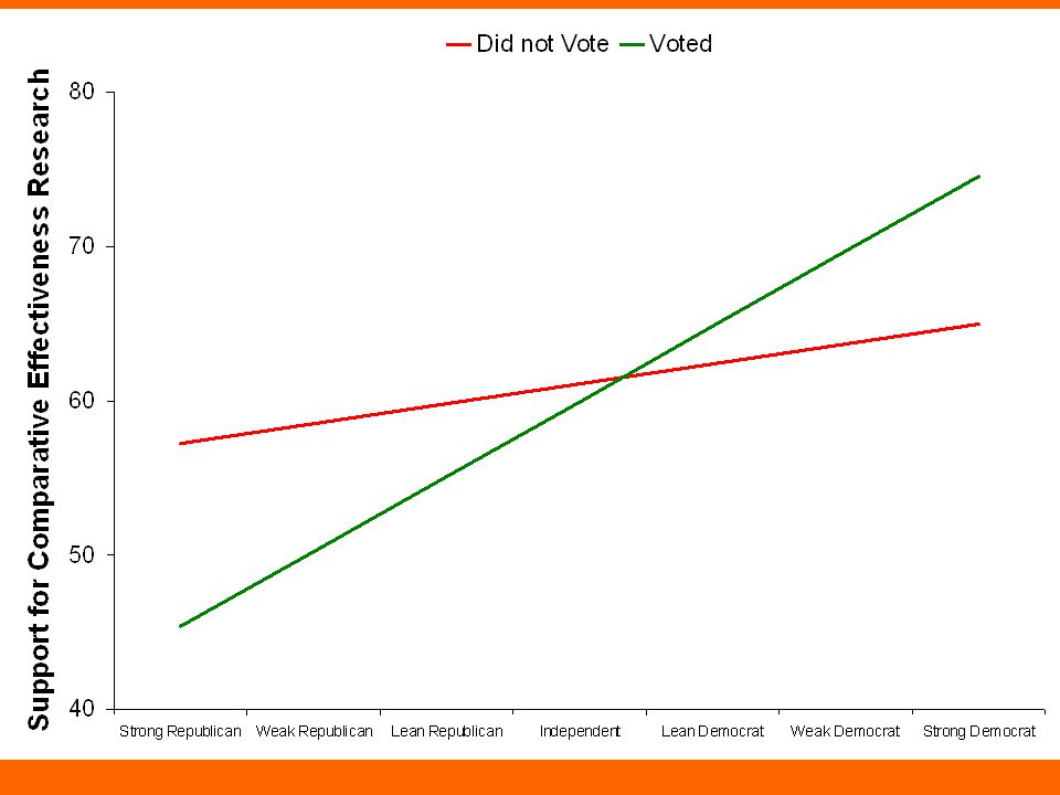
Was CER turned into a partisan issue by political rhetoric? CER seems like it might be a “technocratic” rather than partisan issue… but this survey was conducted in 2009… what was going on? For whom will the relationship between party affiliation and support for CER be strongest? Let’s use “voted in 2008” as a proxy for political engagement (those who didn’t vote probably weren’t paying attention) –Expected relationship between Party affiliation and CER… …for non-voters? …for voters?
 –Expected relationship between Party affiliation and CER… …for non-voters. …for voters .")
22
Coef.SETP Party Affiliation (-3=strong R; 3=strong D)4.5580.25717.7600.000 Voted in 20080.4191.4340.2900.770 Constant59.6311.30945.5400.000 Coef.SETP Party Affiliation (-3=strong R; 3=strong D)1.2860.8781.4600.143 Voted in 2008-1.1381.484-0.7700.443 Party Affiliation x Voted in 20083.5750.9183.9000.000 Constant61.1001.35844.9800.000 61.100 + 1.286*Party – 1.138*Voted + 3.575*Party*Voted + u
 Voted in Constant Coef.SETP Party Affiliation (-3=strong R; 3=strong D) Voted in Party Affiliation x Voted in Constant *Party – 1.138*Voted *Party*Voted + u")
23
Party Aff.VotedParty Aff.VotedParty x VotedConstantPredicted Value Coefficients 1.286-1.1383.57561.100 -30-3.8580061.10057.242 -20-2.5720061.10058.528 0-1.2860061.10059.814 000.0000061.100 101.2860061.10062.386 202.5720061.10063.672 303.8580061.10064.959 Party Aff.VotedParty Aff.VotedParty x VotedConstantPredicted Value Coefficients 1.286-1.1383.57561.100 -31-3.858-1.13775-10.725861.10045.378 -21-2.572-1.13775-7.150561.10050.240 1-1.286-1.13775-3.5752561.10055.101 010.000-1.13775061.10059.962 111.286-1.137753.57525261.10064.824 212.572-1.137757.15050461.10069.685 313.858-1.1377510.7257661.10074.547

25
Notes and Next Time Homework 2 is due on Thursday (11/18) Pick up Homework 3 today. It is due on the Tuesday after Fall Break. Next time: –The “why” and “how” of experiments in political science

Similar presentations


>")
 Answering Political Questions with Quantitative Data (political variables, review of bivariate.>")


>")

 Part I: Interactions Wrap-up Part II: Why Experiment in Political Science?>")

 Review.>")


 Review>")


