1. Intro to Statistics for the Behavioral Sciences PSYC 1900 Lecture 7: Interactions in Regression

2. Bivariate Regression Review Predicts values of Y as a linear function of X Predicts values of Y as a linear function of X The intercept: a The intercept: a The predicted value of Y when X=0 The predicted value of Y when X=0 The slope: b The slope: b The change in Y associated with a one unit change in X The change in Y associated with a one unit change in X Regression line is one that minimizes errors Regression line is one that minimizes errors

3. Partitioning Variance Total variance of Y is partitioned into portion explained by X and error Total variance of Y is partitioned into portion explained by X and error R 2 is portion that is explained R 2 is portion that is explained Standard error of estimate is average deviation around prediction line Standard error of estimate is average deviation around prediction line

4. Hypothesis Testing in Regression The null hypothesis is simply that the slope equals zero. The null hypothesis is simply that the slope equals zero. This is equivalent to testing  =0 in correlation. This is equivalent to testing  =0 in correlation. If the correlation is significant, so must the slope be. If the correlation is significant, so must the slope be. The actual significance of the slope is tested using a t-distribution. The actual significance of the slope is tested using a t-distribution. The logic is similar to all hypothesis testing. The logic is similar to all hypothesis testing. We compare the magnitude of the slope (b) to its standard error (i.e., the variability of slopes drawn from a population where the null is true). We compare the magnitude of the slope (b) to its standard error (i.e., the variability of slopes drawn from a population where the null is true).

5. Hypothesis Testing in Regression The formula to calculate the t value is: The formula to calculate the t value is: Note that standard error of b increases as standard error of the estimate increases Note that standard error of b increases as standard error of the estimate increases We then determine how likely it would be that we found a slope as large as we did using a t distribution (similar to the normal distribution). We then determine how likely it would be that we found a slope as large as we did using a t distribution (similar to the normal distribution).

6. Multiple Regression Allows analysis of more than one independent variable Allows analysis of more than one independent variable Explains variance in Y as a function of a linear composite of iv’s Explains variance in Y as a function of a linear composite of iv’s Each iv has a regression coefficient which provides an estimate of its independent effects. Each iv has a regression coefficient which provides an estimate of its independent effects.

7. Example Let’s examine applicant attractiveness as a function of GREV, Letters of Rec, & Personal Statements Let’s examine applicant attractiveness as a function of GREV, Letters of Rec, & Personal Statements Letters & statements rated on 7pt scales; Y on 10pt. Letters & statements rated on 7pt scales; Y on 10pt. Thus, the predicted evaluation for someone with a great statement (7), ok letters (5), and solid GREV (700) would be: Thus, the predicted evaluation for someone with a great statement (7), ok letters (5), and solid GREV (700) would be:

8. Standardized Regressions The use of standardized coefficients allows easier comparisons of the magnitude of effects The use of standardized coefficients allows easier comparisons of the magnitude of effects Coefficients refer to changes in predicted z-scores of Y as a function of z-scores of x Coefficients refer to changes in predicted z-scores of Y as a function of z-scores of x What is the relation of  to r here? What is the relation of  to r here? In multiple regression,  only equals r if all iv’s are uncorrelated. In multiple regression,  only equals r if all iv’s are uncorrelated.

9. Testing Hypotheses for Individual Predictors Hypothesis testing here is quite similar to that for the single iv in bivariate regression. Hypothesis testing here is quite similar to that for the single iv in bivariate regression. But note that in multiple regression, the standard error is sensitive to the overlap (i.e., correlation) among coefficients. But note that in multiple regression, the standard error is sensitive to the overlap (i.e., correlation) among coefficients. As the intercorrelation increases, so does the standard error. As the intercorrelation increases, so does the standard error.

10. Refining a Model When you are building a model, one way to determine if the addition of new variables improves fit is to see if adding them results in a significant change in R 2. When you are building a model, one way to determine if the addition of new variables improves fit is to see if adding them results in a significant change in R 2. If so, this means that adding the variable explains a significant amount of previously unexplained variability. If so, this means that adding the variable explains a significant amount of previously unexplained variability.

11. Analyzing Interactions in Multiple Regression Many times, we are not only interested in the direct effects of single independent variables on a dependent variable, but also in how one variable may affect the influence of another. That is, how the influence of one independent variable changes as a function of change on a second independent variable. In regression, we represent interactions by using cross-product terms. The unique effect of a cross-product term (i.e., it’s effect after being partialled for the main effects) represents the interaction effect. To achieve this end, we must have the single independent variables that comprise the cross-product in the regression equation.

12. An Example Let’s say we have a 2 (Gender) X 2 (Self-Esteem: High/Low) study on aggression. Aggression is defined as the level of shock given to a confederate in the experimental task. Gender will be scored 0 for males, 1 for females. Self-Esteem will be scored 0 for low, 1 for high (based on a median split of scores). To create the interaction term, we simply multiply scores for gender X self- esteem. Groupgenderself-esteemInteraction Male/LoSE000 Male/HiSE010 Female/LoSE100 Female/HiSE111

13. Our “main-effects” regression equation is: To examine the interaction, we add the cross-product term: If b 3 is significant (or equivalently if the change in R 2 is significant), the interaction is significant. Note: when an interaction is present, it becomes tenuous to interpret the main effects from the first equation. The main effect parameters from the second equation are not easily interpretable.

14. The resulting data from the sample we have provides the following estimates for the first equation: Let’s calculate the predicted values (means) for the groups. LSEmen=6.95, HSEmen=3.78, LSEwomen=4.96, HSEwomen=1.79 Now, we add the interaction term and find:

15. To depict the interaction, we show different regression lines based on 1 iv as a function of the other iv. For men: For women: So, it’s clear that SE has a stronger association with aggression for men than for women.

16. The same can be done with a continuous iv (or iv’s). In this case, the cross-product term will not simply be 1’s and 0’s, but will function in the same manner. To depict the interaction, you should select three different levels of the continuous iv (usually –1sd, the mean, and +1sd). For example, if we use self-esteem scores rather than dichotomize them, the regression equation becomes: You could then show how the effect of gender differs as a function of self-esteem (though in the present case, it might make more sense just to have two lines for gender and show how the effect of self-esteem differs).

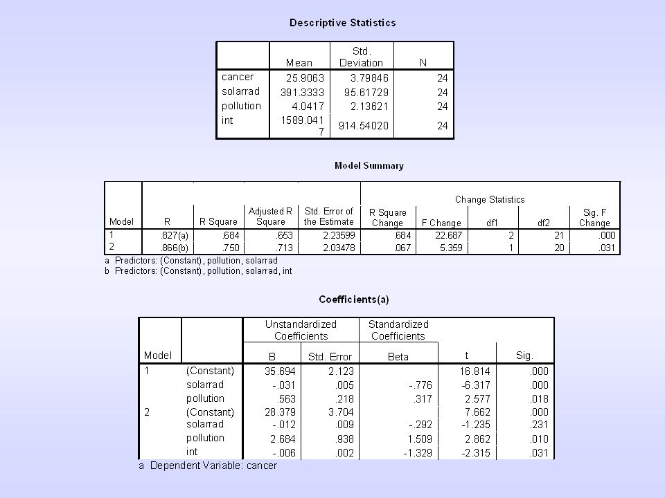
17. An Example Returning to the solar radiation data, we know that increasing sun exposure is associated with decreased breast cancer. Returning to the solar radiation data, we know that increasing sun exposure is associated with decreased breast cancer. What about the role of toxins in the environment? Might it affect this relation? What about the role of toxins in the environment? Might it affect this relation?

19. Top line is plotted substituting +1sd for pollution Bottom line is plotted substituting -1sd for pollution You can see that the benefits of sun exposure decline with increasing exposure to toxins.