Download presentation
Presentation is loading. Please wait.

1
Probabilistic modelling in computational biology Dirk Husmeier Biomathematics & Statistics Scotland

2
James Watson & Francis Crick, 1953

3
Frederick Sanger, 1980

7
Network reconstruction from postgenomic data

8
Model Parameters q

9
Friedman et al. (2000), J. Comp. Biol. 7, 601-620 Marriage between graph theory and probability theory

10
Bayes net ODE model

11
Model Parameters q Probability theory Likelihood

12
Model Parameters q Bayesian networks: integral analytically tractable!

13
UAI 1994

14
Identify the best network structure Ideal scenario: Large data sets, low noise

15
Uncertainty about the best network structure Limited number of experimental replications, high noise

16
Sample of high-scoring networks

17
Feature extraction, e.g. marginal posterior probabilities of the edges High-confident edge High-confident non-edge Uncertainty about edges

18
Number of structures Number of nodes Sampling with MCMC

19
Madigan & York (1995), Guidici & Castello (2003)
, Guidici & Castello (2003)")
21
Overview Introduction Limitations Methodology Application to morphogenesis Application to synthetic biology

22
Homogeneity assumption Interactions don’t change with time

23
Limitations of the homogeneity assumption

24
Example: 4 genes, 10 time points t1t1 t2t2 t3t3 t4t4 t5t5 t6t6 t7t7 t8t8 t9t9 t 10 X (1) X 1,1 X 1,2 X 1,3 X 1,4 X 1,5 X 1,6 X 1,7 X 1,8 X 1,9 X 1,10 X (2) X 2,1 X 2,2 X 2,3 X 2,4 X 2,5 X 2,6 X 2,7 X 2,8 X 2,9 X 2,10 X (3) X 3,1 X 3,2 X 3,3 X 3,4 X 3,5 X 3,6 X 3,7 X 3,8 X 3,9 X 3,10 X (4) X 4,1 X 4,2 X 4,3 X 4,4 X 4,5 X 4,6 X 4,7 X 4,8 X 4,9 X 4,10
 X 1,1 X 1,2 X 1,3 X 1,4 X 1,5 X 1,6 X 1,7 X 1,8 X 1,9 X 1,10 X (2) X 2,1 X 2,2 X 2,3 X 2,4 X 2,5 X 2,6 X 2,7 X 2,8 X 2,9 X 2,10 X (3) X 3,1 X 3,2 X 3,3 X 3,4 X 3,5 X 3,6 X 3,7 X 3,8 X 3,9 X 3,10 X (4) X 4,1 X 4,2 X 4,3 X 4,4 X 4,5 X 4,6 X 4,7 X 4,8 X 4,9 X 4,10")
25
Supervised learning. Here: 2 components t1t1 t2t2 t3t3 t4t4 t5t5 t6t6 t7t7 t8t8 t9t9 t 10 X (1) X 1,1 X 1,2 X 1,3 X 1,4 X 1,5 X 1,6 X 1,7 X 1,8 X 1,9 X 1,10 X (2) X 2,1 X 2,2 X 2,3 X 2,4 X 2,5 X 2,6 X 2,7 X 2,8 X 2,9 X 2,10 X (3) X 3,1 X 3,2 X 3,3 X 3,4 X 3,5 X 3,6 X 3,7 X 3,8 X 3,9 X 3,10 X (4) X 4,1 X 4,2 X 4,3 X 4,4 X 4,5 X 4,6 X 4,7 X 4,8 X 4,9 X 4,10
 X 1,1 X 1,2 X 1,3 X 1,4 X 1,5 X 1,6 X 1,7 X 1,8 X 1,9 X 1,10 X (2) X 2,1 X 2,2 X 2,3 X 2,4 X 2,5 X 2,6 X 2,7 X 2,8 X 2,9 X 2,10 X (3) X 3,1 X 3,2 X 3,3 X 3,4 X 3,5 X 3,6 X 3,7 X 3,8 X 3,9 X 3,10 X (4) X 4,1 X 4,2 X 4,3 X 4,4 X 4,5 X 4,6 X 4,7 X 4,8 X 4,9 X 4,10.")
26
Changepoint model Parameters can change with time

27
Changepoint model Parameters can change with time

28
t1t1 t2t2 t3t3 t4t4 t5t5 t6t6 t7t7 t8t8 t9t9 t 10 X (1) X 1,1 X 1,2 X 1,3 X 1,4 X 1,5 X 1,6 X 1,7 X 1,8 X 1,9 X 1,10 X (2) X 2,1 X 2,2 X 2,3 X 2,4 X 2,5 X 2,6 X 2,7 X 2,8 X 2,9 X 2,10 X (3) X 3,1 X 3,2 X 3,3 X 3,4 X 3,5 X 3,6 X 3,7 X 3,8 X 3,9 X 3,10 X (4) X 4,1 X 4,2 X 4,3 X 4,4 X 4,5 X 4,6 X 4,7 X 4,8 X 4,9 X 4,10 Unsupervised learning. Here: 3 components

29
Extension of the model q

30
q

31
q k h Number of components (here: 3) Allocation vector
 Allocation vector")
32
Analytically integrate out the parameters q k h Number of components (here: 3) Allocation vector
 Allocation vector")
34
P(network structure | changepoints, data) P(changepoints | network structure, data) Birth, death, and relocation moves RJMCMC within Gibbs
 P(changepoints | network structure, data) Birth, death, and relocation moves RJMCMC within Gibbs")
35
Dynamic programming, complexity N 2

37
Collaboration with the Institute of Molecular Plant Sciences at Edinburgh University (Andrew Millar’s group) - Focus on: 9 circadian genes: LHY, CCA1, TOC1, ELF4, ELF3, GI, PRR9, PRR5, and PRR3 - Transcriptional profiles at 4*13 time points in 2h intervals under constant light for - 4 experimental conditions Circadian rhythms in Arabidopsis thaliana
 - Focus on: 9 circadian genes: LHY, CCA1, TOC1, ELF4, ELF3, GI, PRR9, PRR5, and PRR3 - Transcriptional profiles at 4*13 time points in 2h intervals under constant light for - 4 experimental conditions Circadian rhythms in Arabidopsis thaliana")
38
Comparison with the literature Precision Proportion of identified interactions that are correct Recall = Sensitivity Proportion of true interactions that we successfully recovered Specificity Proportion of non-interactions that are successfully avoided

39
CCA1 LHY PRR9 GI ELF3 TOC1 ELF4 PRR5 PRR3 False negative Which interactions from the literature are found? True positive Blue: activations Red: Inhibitions True positives (TP) = 8 False negatives (FN) = 5 Recall= 8/13= 62%
 = 8 False negatives (FN) = 5 Recall= 8/13= 62%.")
40
Which proportion of predicted interactions are confirmed by the literature? False positives Blue: activations Red: Inhibitions True positive True positives (TP) = 8 False positives (FP) = 13 Precision = 8/21= 38%
 = 8 False positives (FP) = 13 Precision = 8/21= 38%.")
41
Precision= 38% CCA1 LHY PRR9 GI ELF3 TOC1 ELF4 PRR5 PRR3 Recall= 62%

42
True positives (TP) = 8 False positives (FP) = 13 False negatives (FN) = 5 True negatives (TN) = 9²-8-13-5= 55 Sensitivity = TP/[TP+FN] = 62% Specificity = TN/[TN+FP] = 81% Recall Proportion of avoided non-interactions
![True positives (TP) = 8 False positives (FP) = 13 False negatives (FN) = 5 True negatives (TN) = 9² = 55 Sensitivity = TP/[TP+FN] = 62% Specificity = TN/[TN+FP] = 81% Recall Proportion of avoided non-interactions](http://images.slideplayer.com/12/3461175/slides/slide_42.jpg "True positives (TP) = 8 False positives (FP) = 13 False negatives (FN) = 5 True negatives (TN) = 9² = 55 Sensitivity = TP/[TP+FN] = 62% Specificity = TN/[TN+FP] = 81% Recall Proportion of avoided non-interactions")
43
Model extension So far: non-stationarity in the regulatory process

44
Non-stationarity in the network structure

45
Flexible network structure.

46
Model Parameters q

47
Use prior knowledge!

48
Flexible network structure.

49
Flexible network structure with regularization Hyperparameter Normalization factor

50
Flexible network structure with regularization Exponential prior versus Binomial prior with conjugate beta hyperprior

51
NIPS 2010

52
Overview Introduction Limitations Methodology Application to morphogenesis Application to synthetic biology

53
Morphogenesis in Drosophila melanogaster Gene expression measurements at 66 time points during the life cycle of Drosophila (Arbeitman et al., Science, 2002). Selection of 11 genes involved in muscle development. Zhao et al. (2006), Bioinformatics 22
, Bioinformatics 22.")
54
Can we learn the morphogenetic transitions: embryo larva larva pupa pupa adult ?

55
Average posterior probabilities of transitions Morphogenetic transitions: Embryo larva larva pupa pupa adult

57
Can we learn changes in the regulatory network structure ?

59
Overview Introduction Limitations Methodology Application to morphogenesis Application to synthetic biology

62
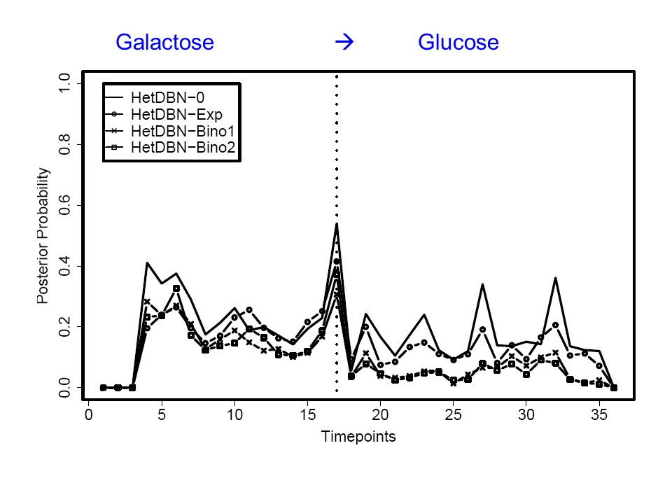
Can we learn the switch Galactose Glucose? Can we learn the network structure?

63
Task 1: Changepoint detection Switch of the carbon source: Galactose Glucose

65
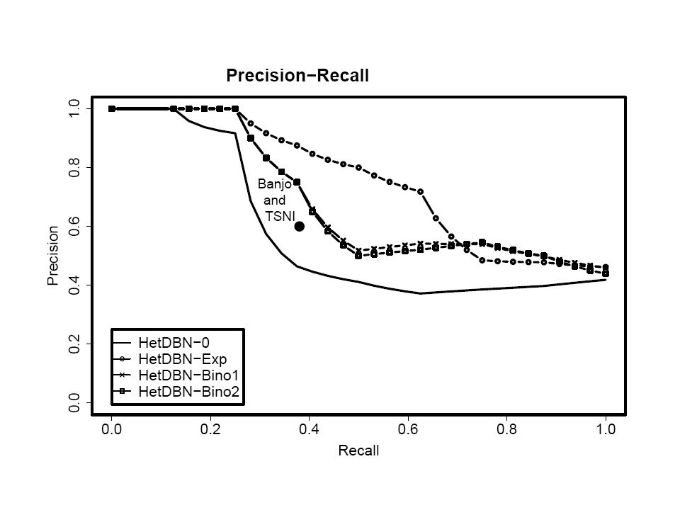
Task 2: Network reconstruction Precision Proportion of identified interactions that are correct Recall Proportion of true interactions that we successfully recovered

66
BANJO: Conventional homogeneous DBN TSNI: Method based on differential equations Inference: optimization, “best” network

68
Sample of high-scoring networks

69
Marginal posterior probabilities of the edges P=1 P=0 P=0.5

70
P=1 True network Thresh0.9 Prec1 Recall1/2 Precision Recall

71
P=1 P=0.5 True network Thresh0.90.4 Prec12/3 Recall1/21 Precision Recall

72
P=1 P=0 P=0.5 True network Thresh0.90.4-0.01 Prec12/31/2 Recall1/211 Precision Recall

74
Future work

75
How are we getting from here …

76
… to there ?!

77
Input: Learn: MCMC Prior knowledge

Similar presentations


 11/05/07. Methods Linear –PCA (Raychaudhuri et al. 2000) –NIR (Gardner et al. 2003) Nonlinear –Bayesian network (Friedman.>")


>")
