1. Introduction to computational plasma physics
雷奕安

2. 课程概况 http://www.phy.pku.edu.cn/~fusion/forum/viewtopic.php?t=77 上机
成绩评定为期末大作业

3. Related disciplines Computation fluid dynamics (CFD)
Applied mathematics, PDE, ODE
Computational algorithms
Programming language, C, Fortran
Parallel programming, OpenMP, MPI
Plasma physics, space, fusion, …
Unix, Linux, …

5. 大规模数值模拟的特殊性 数值计算 数值模拟 大规模数值模拟 数学问题 算法 编程 物理问题 数学模型 算法编程 物理问题及数学模型
相关学科研究人员支持
超级计算机软硬件系统

6. Contents What is plasma Basic properties of plasma
Plasma simulation challenges
Simulation principles

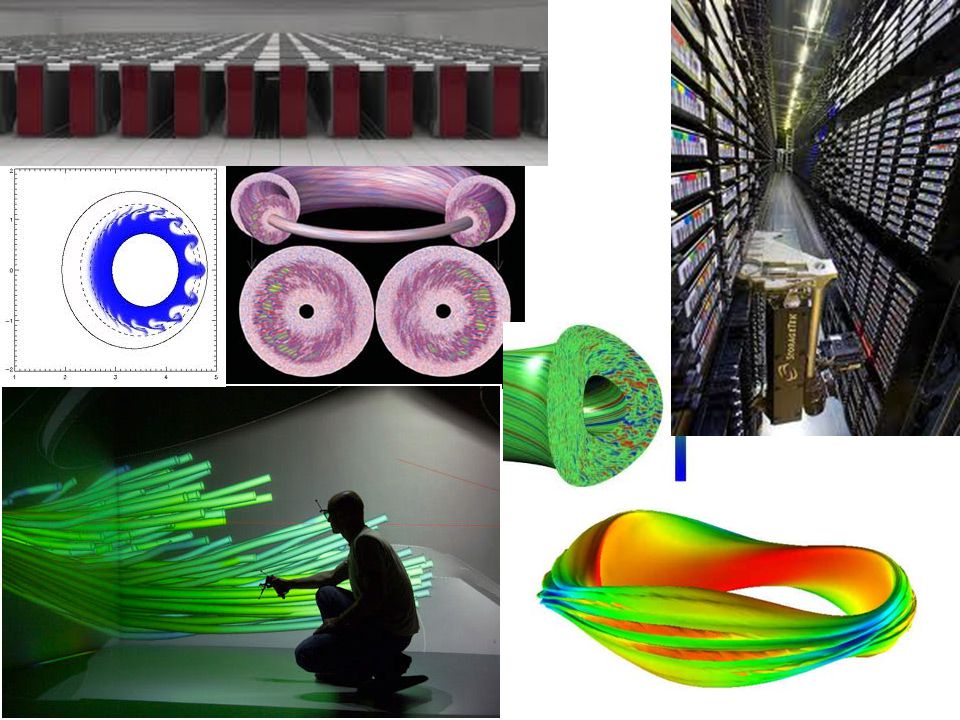
7. What is plasma Partially ionized gas, quasi-neutral Widely existed
Fire, lightning, ionosphere, polar aurora
Stars, solar wind, interplanetary (stellar, galactic) medium, accretion disc, nebula
Lamps, neon signs, ozone generator, fusion energy, electric arc, laser-material interaction
Basic properties
Density, degree of ionization, temperature, conductivity, quasi-neutrality
magnetization

8. Plasma vs gas Property Gas Plasma Conductivity Very low, insulator
Very high, conductor
Species
Usually one
At least two, ion, electron
Distribution
Usually Maxwellian
Usually non-Maxwellian
Interaction
Binary, short range
Collective, long range

10. Basic properties Temperature Quasi-neutrality Thermal speed
Plasma frequency
Plasma period

11. Debye length λD
U→0
System size and time
Debye shielding

12. Debye lengths

13. Plasma parameter
Strong coupling
Weak coupling

14. Weakly coupled plasmas

15. Collision frequency Mean-free-path Collisional plasma (Collisionless)
Collisioning frequency

16. Magnetized plasma Anisotropic Gyroradius Gyrofrequency
Magnetization parameter
Plasma beta

17. Simulation challenges
Problem size: 1014 ~ 1024 particles
Debye sphere size: 102 ~ 106 particles
Time steps: 104 ~ 106
Point particle, computational unstable, sigularities

18. Solution No details, essence of the plasma
One or two dimension to reduce the size
No high frequency phenomenon, increase time step length
Reduce ND, mi / me
Smoothing particle charge, clouds
Fluidal approaches, single or double
Kinetic approaches, df/f

19. Simple Simulation Electrostatic 1 dimensional simulation, ES1
Self and applied electrostatic field
Applied magnetic field
Couple with both theory and experiment, and complementing them

20. Basic model

21. Basic model

22. Basic model Field -> force -> motion -> field -> …
Field: Maxwell's equations
Force: Newton-Lorentz equations
Discretized time and space
Finite size particle
Beware of nonphysical effects

23. Computational cycle

24. Equation of motion vi, pi, trajectory
Integration method, fastest and least storage
Runge-Kutta
Leap-frog
cp]$ cat b.f90
program abc
!implicit double precision (a-h,o-z)
x0 = 1
vx0 = 0
y0 = 0
vy0 = 1
!dt = 0.05
read (*,*) dt
N = 30/dt
do i = 0, N+3
x1 = x0 + vx0*dt
y1 = y0 + vy0*dt
r = sqrt(x0*x0 + y0*y0)
fx = -x0/r**3
fy = -y0/r**3
vx1 = vx0 + fx*dt
vy1 = vy0 + fy*dt
! if(mod(i,N/10).eq.2)
write(*,*) x0, y0, -1/r+(vx0*vx0+vy0*vy0)/2
x0 = x1; y0 = y1; vx0 = vx1; vy0 = vy1
enddo
end
cp]$ cat c.f90
N = 50/dt
xh0 = (x0+x1)/2; yh0 = (y0+y1)/2
do i = 0, N
xh1 = xh0+vx0*dt; yh1 = yh0 + vy0*dt;
r = sqrt(xh0*xh0 + yh0 *yh0 )
fx = -xh1/r**3
fy = -yh1/r**3
! if(mod(i,N/100).eq.0)
write(*,*) xh0, yh0, -1/r+(vx0*vx0+vy0*vy0)/2
xh0 = xh1; yh0 = yh1; vx0 = vx1; vy0 = vy1

25. Planet Problem Forward differencing x0 = 1; vx0 = 0; y0 = 0; vy0 = 1
read (*,*) dt
N = 30/dt
do i = 0, N+3
x1 = x0 + vx0*dt
y1 = y0 + vy0*dt
r = sqrt(x0*x0 + y0*y0)
fx = -x0/r**3
fy = -y0/r**3
vx1 = vx0 + fx*dt
vy1 = vy0 + fy*dt
! if(mod(i,N/10).eq.2)
write(*,*) x0, y0, -1/r+(vx0*vx0+vy0*vy0)/2
x0 = x1; y0 = y1; vx0 = vx1; vy0 = vy1
enddo
end
Forward differencing

26. Planet Problem ./a.out > data 0.1 $ gnuplot
Gnuplot> plot “data” u 1:2

27. Planet Problem ./a.out > data 0.01 $ gnuplot
Gnuplot> plot “data” u 1:2

28. Planet Problem Leap Frog x0 = 1; vx0 = 0; y0 = 0; vy0 = 1
read (*,*) dt
N = 30/dt
x1 = x0 + vx0*dt
y1 = y0 + vy0*dt
xh0 = (x0+x1)/2; yh0 = (y0+y1)/2
do i = 0, N
xh1 = xh0+vx0*dt; yh1 = yh0 + vy0*dt;
r = sqrt(xh0*xh0 + yh0 *yh0 )
fx = -xh1/r**3
fy = -yh1/r**3
vx1 = vx0 + fx*dt
vy1 = vy0 + fy*dt
! if(mod(i,N/100).eq.0)
write(*,*) xh0, yh0, -1/r+(vx0*vx0+vy0*vy0)/2
xh0 = xh1; yh0 = yh1; vx0 = vx1; vy0 = vy1
enddo
end
Leap Frog

29. Planet Problem ./a.out > data 0.1 $ gnuplot
Gnuplot> plot “data” u 1:2

30. Planet Problem ./a.out > data 0.01 $ gnuplot
Gnuplot> plot “data” u 1:2

31. Field equations
Poisson’s equation

32. Field equations Poisson’s equation is solvable
In periodic boundary conditions, fast Fourier transform (FFT) is used, filtering the high frequency part (smoothing), is easy to calculate

33. Particle and force weighting
Particle positions are continuous, but fields and charge density are not, interpolating
Zero-order weighting
First-order weighting, cloud-in-cell

36. Higher order weighting
Quadratic or cubic splines, rounds of roughness, reduces noise, more computation

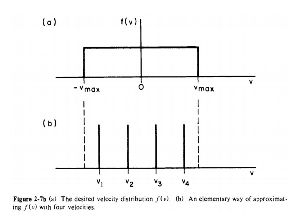
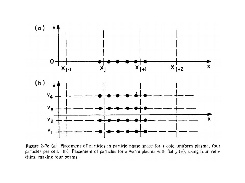
37. Initial values Number of particles and cells Weighting method
Initial distribution and perturbation
The simplest case: perturbed cold plasma, with fixed ions.
Warm plasma, set velocities

40. Initial values

41. Diagnostics Graphical snapshots of the history x, v, r, f, E, etc.
Not all ti
For particle quantities, phase space, velocity space, density in velocity
For grid quantities, charge density, potential, electrical field, electrostatic energy distribution in k space

42. Tests Compare with theory and experiment, with answer known
Change nonphysical initial values (NP, NG, Dt, Dx, …)
Simple test problems

43. Server connection Ssh Host: 162.105.23.110, protocol: ssh2
Your username & password
Vnc connection In ssh shell: “vncserver”, input vnc passwd, remember xwindow number
Tightvnc: :xx (the xwindow number)
Kill vncserver: “vncserver –kill :xx” (x-win no.)

44. Xes1 Xes1 document Xgrafix already compiled in /usr/local
Xes1 makefile
make
./xes1 -i inp/ee.inp
LIBDIRS = -L/usr/local/lib -L/usr/lib -L/usr/X11R6/lib64

45. Clients
Ssh putty.exe
Vncviewer
Pscp: