1. Welcome to John Costain’s Peak Oil Website This PowerPoint presentation is an ongoing effort by me to try to understand for myself the current debate on when the year of World Peak Oil will occur. Will it be in the year 2026 (USGS) or is it happening now in 2006 (Deffeyes and others)? Data-driven comments to costain@vt.edu are welcome. Copyright 2006 by John Costain. Permission to use this presentation in classrooms or before governmental agencies is freely granted. Version 1.4, April 29, 2006

2. The U.S. and World Oil Peaks What M. King Hubbert did to predict them and how to do it yourself Prepared by John K. Costain Department of Geosciences Virginia Tech Blacksburg, VA

3. Acknowledgements http://math.fullerton.edu/mathews/N310/projects/p4.htm Population Model http://www.princeton.edu/hubbert/ Peak Oil, Prof. Kenneth S. Deffeyes http://tonto.eia.doe.gov/dnav/pet/hist/mcrfpus1A.htm U. S. Oil Production Data

4. Two methods can be used to compute Hubbert’s curves 1. The “Population Model” 2. Deffeyes Method

5. P = oil production per year Q = accumulated oil production So Q(t) = all oil produced up to and including time, t That is, Q(1) = P(1) Q(2) = P(1) +P(2) Q(3) = P(1) +P(2) + P(3) etc. Definitions

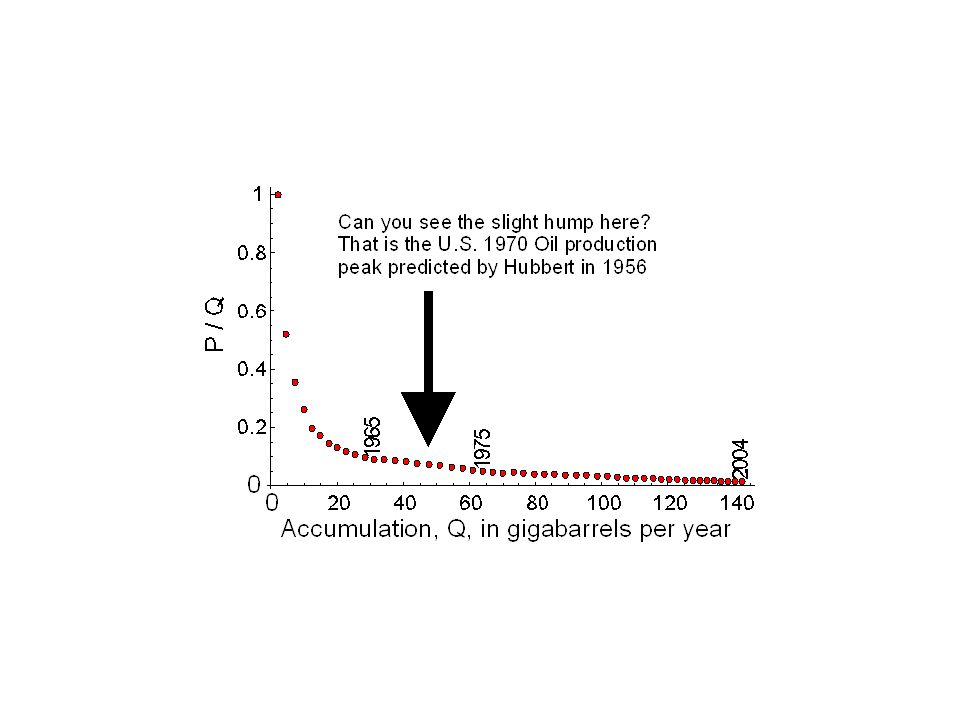
6. Plot the ratio P/Q versus Q First point, where P = Q Accumulation, Q, in gigabarrels U.S. Oil Production Data from: http://www.eia.doe.gov/emeu/aer/petro.html 0 0 Note the total: 140,000,000,000 The EIA is the Energy Information Administration, the statistical information collection and analysis branch of the U.S. Department of Energy. P is oil production in gigabarrels Q is oil accumulation in gigabarrels

8. Now, just where the line is straight P/ Q = m Q + b dQ / dt = Q’ = b Q + m Q 2 First, get the general solution of the differential equation P = dQ / dt = b Q + m Q 2 Let Mathematica solve this. solution = DSolve [ Q’ [ t ] == b Q [ t ] + m Q [ t ]^2, Q [ t ], t ] ; Q(t) = = Where m and b are determined from the data The Details Note that Q(t) =P ( t ) d t So d Q(t) / d t = P(t) ( because we got Q by adding up P ) So dQ / dt = P = b Q + m Q 2

9. Q(t) = This is the general solution for accumulation Q(t) as a function of time t. All we need are the constants m and b, which we get from the least-squares fit of the straight line segment, and the constant of integration, C[1], which we get by knowing a value of Q(t) at time t and the observed values of m and b. and then we can plot the accumulation Q(t) versus time t. The Details (continued) =

10. Fit a straight line y = m x + b to the linear portion of the curve. P / Q = m Q + b P = m Q + b Q 2 But Q(t) is P ( t ) d t So d Q(t) / d t = P(t) d Q / d t = m Q + b Q 2 This is the differential equation that we need to solve ( because we got Q by adding up P ) It is also called “The Population Model” Q(t) is called the “logistic function”. The derivative of Q(t) is called the Hubbert curve

11. It is important to note that the definition d Q / d t = P makes this analysis exact. No assumptions about what kind of a curve should be fitted to the data are necessary or even justifiable.

12. First find the values of the constants m and b over the interval of the red straight line. Fit a straight line to points on the curve For example, choose the interval 1984 - 2004 U.S. Oil Production

13. Let Mathematica do the fit. For example : fit [ x_ ] = Fit [Take [Transpose [ { CumulatedUSTotalProduction, USTotalProduction / CumulatedUSTotalProduction }], { FirstPoint, LastPoint } ], {1, x}, x] Let FirstPoint correspond to the year 1984 Let LastPoint correspond to the year 2004 The resulting least-squares fit is 0.0587093 - 0.000257955 x For x = the oil accumulation in 1984 P / A = 0.022533 For x = the oil accumulation in 2004 P / A = 0.00959897 The U.S. ratio of the annual production to accumulation (P/Q) decreased from 0.022533 (2.25%) in 1984 to 0.00959897 (0.96%) in 2004. So m = - 0.000257955 b = 0.0587093

14. Intuitively, it is clear at this point that if you know the rate of change of annual oil production and the equation of the oil production curve (the derivative of the logistic equation) then you can predict future production values from past values. What is the principal uncertainty ? It is the slope of that straight line. If you tell me that future production can change the slope of that straight line then, of course, future oil production will increase. So later we need to look at what it takes to change the slope of the straight line.

15. Result of fitting a straight line from 1984 - 2004

16. The good fit suggests that the “Population Model” is valid

17. This is called a “Hubbert Curve”. It is the derivative of the accumulation curve. It is symmetric about the peak and therefore at the time of the peak you will have produced one-half of all the oil that will be produced. ½ of oil produced ½ of oil yet to be produced

18. Deffeyes (2005) deduced a clever, simpler method that does not require the solution of a differential equation. As before, just where the line is straight P/ Q = m Q + b where m and b are again determined from the data in the same way.

19. P / Q = m Q + b P = m Q 2 + b Q When P = 0, Q = Q T = - b / m so m = - b / Q T P = ( - b / Q T ) Q 2 + b Q P = b (- Q 2 / Q T + Q ) The Details P = b Q ( 1 - Q / Q T ) The term Q / Q T is the fraction of total oil Q T that has already been produced and the term (1 - Q / Q T ) is the fraction yet to be produced.

20. P = b Q ( 1 - Q / Q T ) But the equation has no time, t, in it. You can’t plot P versus t because it is an equation of P versus Q, not t. Here Deffeyes cleverly shows how to get P versus time. We know what the accumulation Q is at the Year 2004. It is 190.383409 gigabarrels. The Details (continued) We are going to determine the production times that would have occurred if we were to compute the times between each 1 gigabarrel of production instead of using the time of 1 year between what was the actual production.

21. YearsPerGigabarrel = 1 / GigabarrelsPerYear; t = Table [ 0, { Round [ - b/m] }]; n = Round[Last[CumulatedUSTotalProduction]] ; = Round[190.383] = 190 t [[n]] = Last [year] ; = 2004 Do [ D t=YearsPerGigabarrel[[i]]; t [[i - 1]] = t [[i]] - D t,{i,n,2, - 1}]; Do [ D t=YearsPerGigabarrel[[i]]; t [[i+1]] = t [[i]] + D t,{i,n,Qt - 1,1}]; year[[ ]] is where the known production years are stored. t [[ ]] = the desired new times in fractional years per gigabarrel. D t = the time (in years) between each successive gigabarrel of production n = the number of “Years per Gigabarrel” times. Qt = the accumulated oil when there is no more production = - b/m The Details (continued) The desired times are in t.

22. Now it is possible to plot production versus time and to compare Deffeyes’ method with the Population Model. P(t) = b Q ( 1 - Q / Q T ) where P(t) is in gigabarrels per year and adjacent Qs differ from each other by exactly 1 gigabarrel.

24. Using the Population Model one can try to predict future gas prices Note that there is no point of inflection in the solution (red line) to the differential equation. There will therefore be no peak in the price of gasoline. That is, the price of gas will continue to rise. Part 1.

25. Gasoline price, not adjusted for Inflation Year Accumulation Cumulated gasoline prices Ratio Part 2.

26. Gasoline price, adjusted for Inflation Year Digression: Gasoline prices adjusted for inflation! Source: American Petroleum Institute

27. This line segment Gives this Hubbert curve Accumulation, QYear P/Q The red line segment is all you need to know to generate Hubbert’s curves or to make predictions about the impact of new oil fields or the contribution of better secondary recovery methods. (or any other segment with the same slope and intercept)

28. What did Hubbert do in 1956 to predict the 1970 oil peak?

29. Accumulation, Q This interval possibly used by Hubbert in 1956 to predict the U.S. oil peak in 1970. Hubbert’s Prediction of the 1970 U.S. Oil Peak P / Q 25 50 75 100 125 150 175 200 0.02 0.04 0.06 0.08 1 9 3 3 1 9 5 7 Alaska production omitted This segment gives this Hubbert curve

30. Note: Over this entire time period the price of gasoline has been increasing and decreasing with little affect on the shape of the Hubbert curve.

31. 185018751900192519501975200020252050 0.5 1 1.5 2 2.5 3 With Alaska (1976.47) Without Alaska (1971.77) Alaska production delayed the U.S. Oil Peak by 4.7 years Oil production, gigabarrels Year Production from Alaskan oil delayed the onset of the U.S. Oil Peak by 4.7 years. The same size oil field would have a much smaller effect on postponing the time of the World Oil Peak because there is so much more oil produced by the entire world. See a subsequent slide for the amount of delay using Alaska as an example.

32. The World Oil Peak

33. The United States already has felt briefly the importance of peak. Precisely, as forecast by Hubbert in 1956 (either ignored, or regarded in gross error by most people at the time), U. S. oil production peaked in 1970. The United States actually had to begin to import oil about 15 years before the peak was reached, as demand already had outstripped production capacity by peak production time. The fact that U. S. production had peaked in 1970, and then began to decline further assured the success of the Arab oil embargo against the United States in 1973, and altered U. S.-Middle East foreign policy. The United States well past its peak of oil production, now imports more oil than it produces. When world oil production peaks, there will be nowhere else for the world to go for more oil. The problem then will become the harsh reality of distribution of an irreversibly declining resource, rather than dividing more and more oil, as has been the pleasant experience to the present. This is when final competition begins for the last half of world oil reserves. It will be a global struggle. All countries will be involved —the industrialized countries more so than the less developed countries. For the first time, the entire world will be locked in one massive contest for a single resource. This may be the most important event in human history. In terms of lifestyles, our relatively cheap and abundant food supplies, the manufacture of many things, which depend on the energy of oil, and the distribution of these products, the beginning of the decline of oil production will be a momentous event. Encircling the Peak of World Oil ProductionEncircling the Peak of World Oil Production

34. This is the shape of all of the solutions to the differential equation. 1920194019601980200020202040 50 100 150 200 This is called a “logistic curve”. Time Accumulation, Q(t), of oil production Here the slope reaches a maximum and then decreases. That corresponds to the time of the peak in the Hubbert curve. The Hubbert curve is the derivative of this curve. A logistic curve is “an S -shaped curve that describes population growth as a function of time. When the population is low, growth begins slowly, then becomes rapid and increases exponentially, finally slowing down and reaching equilibrium as the population reaches the maximum that the environment can support.

35. What does the actual world oil accumulation data show? Of course we don’t know the future accumulation or how it will deviate from the imposed symmetry shown above. Can we overcome the statistics by discovering new fields, by using better secondary recovery methods, etc.?

36. This notebook with these figures by Eric W. Weisstein can be downloaded from http://mathworld.wolfram.com/notebooks/DifferentialEquations/LogisticEquation.nb. x(t) = Q(t) = the accumulation = 1 ( ) 1 x0x0 1 + - 1 e - r t The quantity r is a rate and is the same as our intercept b. For a given value of r in the examples above, a family of curves is obtained by changing the initial value of the accumulation, that is, x 0 is the initial value of the accumulation at t = 0. Such a pair of values (t, x 0 ) is required to identify the particular member of the family of curves for our value of r=0.005. In the previous slide for our solution we used the (t,Q) pair (2004,1026.05) to solve for C[1]. More on the logistic equation

37. Using the methodology of the “Population Model” we get the following prediction for the World Oil Peak “Remaining conventional, proven world petroleum reserves are estimated to be 2130.5 billion barrels equivalent.” says Arthur E. Berman to Houston Geological Society, June 2005. Berman is Director of Petroleum Reports.com a company that provides petroleum reports and digital maps to the oil and gas industry. This line intersects the x-axis at Q T = 2175 gb, almost exactly (within 2%) of the reserves estimated by Berman (below) using other methods. This agree- ment between the ultimate production predicted by the Hubbert method and the estimated reserves would assume that all of the estimated reserves can be recovered (produced).

38. And the associated Hubbert curve is 30 25 20 15 10 5 P e a k a t y e a r 2 0 0 6. 1 9 18501900195020002050 Year World Oil Peak from Hubbert's theory World oil production in gigabarrels The Hubbert curve is symmetrical. Note that when production declines after the peak there will be more and more data because the amount of accumulated oil increases, so additional production will find it more and more difficult to shift the peak or destroy the symmetry. The more data, the better the Hubbert method works.

39. 5 10 15 20 25 Alaska production delays the World Oil Peak by 2.5 years 185018751900192519501975200020252050 With Alaska Without Alaska 2.5 years Production from Alaskan oil would delay the onset of the World Oil Peak by 2.5 years. The same size oil field has a much smaller effect on the delay of the World Oil Peak because there is so much more oil produced by the entire world. Oil production, gigabarrels Year

40. The big question: Can future oil production change the slope of the black line to reach one of the predictions (3 trillion barrels) made by the U.S.G.S. (red dashed line) ? Background figure from Deffeyes, 2005, Beyond Oil, p. 43. We have essentially reproduced the latest published results of Professor Ken Deffeyes, Beyond Oil: The View from Hubbert’s Peak, 2005, p. 43. The slope of this real- data straight-line seg- ment puts the peak in the year 2006 3000 gigabarrels World Oil Peak 2006 Hubbert prediction

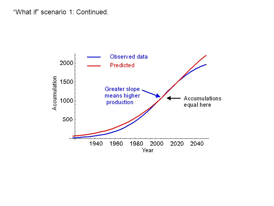
41. “What if” scenario 1: Total oil available to be produced (Q t ) is assumed to be 3000 gb instead of 2000 gb. The slope and intercept both change and an abrupt decrease in present production is required. This is the scenario that would have occurred if we had started off using less oil, and if there were much more oil available to produce. Next slide shows this scenario combined with the 2006 oil peak. Background figure from Deffeyes, 2005, Beyond Oil, p. 43.

42. Accumulations equal here “What if” scenario 1: Continued.

44. The abrupt increase in production D P of 8.3 gb per year is unrealistic. This is the scenario that would have occurred if the annual growth rate were the same, and if there were much more oil available to produce. “What if” scenario 2: Total oil available to be produced is assumed to be 3000 gb instead of 2000 gb. The intercept does not change but the slope does, corresponding to an abrupt increase in present day production. The result: The peak is delayed until the year 2017 Background figure from Deffeyes, 2005, Beyond Oil, p. 43.

45. “What if” scenario 3: Total oil available to be produced Q T is assumed to range from present day estimate (2175 gb) to an ultimate total of 3675 gigabarrels. The intercept and slope both change.

46. What is the meaning of the slope m ? P/Q = m Q + b m must have dimensions of 1/Q because P/Q is dimensionless So from the preceding figure m can be interpreted as: - intercept QTQT = Fraction of Q produced at any time t Q at any time t = % production P per accumulation Q Accumulation Q = constant for any time t for a straight line m = = -b-b QTQT P/Q Q = = a negative number because we are producing less and less as we accumulate more and more

47. The Details

48. If world production/accumulation rate can be reduced from 5.2% to 3.8% then the world oil peak moves out to the year 2029. “What if” scenario 3 continued: Results. We need to start consuming less to move the peak out.

49. Examples of Secondary Recovery (with previous slide superimposed) Magnolia Petroleum Co.’s West Burkburnett field in Texas is an example of the success of a large waterflood secondary-recovery operation. Using a five-spot water-injection program, the company’s flood recovered 9 million bbl (0.009 gb) of oil between 1944 and 1953, or 1.4 times that recovered by primary methods. In Illinois, an initial five-spot program by Adams Oil & Gas Co.-Felmont Corp. in 1943 in the Patoka field, Marion County, resulted in a much more rapid response in the oil production rate than expected. The field, which produced 2.8 million bbl of oil by primary production, produced an additional 6.4 million bbl (0.0064 gb) of waterflood oil by August 1960. In the Bradford field of Pennsylvania, results from an air-injection project were quickly realized. The daily injection of air at an average of 68,600 ft3/well at 300 psi increased per-well production from 0.25 to 12 BOPD in less than two months. Annual production from the 22-well project increased from 3,474 bbl in 1925 to 18,524 (0.0000185 gb) bbl in 1927, and total production from the field is estimated to have increased by 25% from the air injection alone. All from the Society of Petroleum Engineers at http://www.spe.org/

50. How to estimate the effect of additional oil production from secondary recovery, discovery of new oil fields, etc. The quantity Q T, referred to in earlier slides, is the ultimate production when the last drop has been produced. Therefore, it is this quantity that can be changed in the sequence of statements (from an earlier slide): For example, you might decide that instead of Q T =2175 you are justified in saying Q T = 2250. Then rerun the program. No other changes.

51. These are the USGS “bottom-up” predictions. 28 gb 43 gb Where will the required 0.75 gb/year come from? 2006 Assumed growth in production. That is, it is the assumed ability to produce 2% more each year because the oil is there to produce on time. In 30 years, in order to reach 3000 gb, we need to produce 24 gb more, which is almost as much as we have produced for the last 100 years. 0.75 gb/yr 0.77 gb/yr 52 gb Hubbert’s World Oil Peak is here. Background figure from the U.S. Geological Survey World Petroleum Assessment 2000—Description and Results, USGS Digital Data Series DDS-60, Version 1.1, 2000 R/P = Resource/Production ; The “Reserves” are a small fraction of the “Resource”.

53. Observation 1. Data discrepancy.

54. What difference does this discrepancy make? No difference in the year of the peak, which is determined by the slope of the straight-line portion of accumulation versus time. These two curves were computed from the data on the previous slide. The method used was the differential equation of the population model (the Hubbert method), and all data in Table RV-1 (four points) were used. The Mathematica statements are on the following two slides. The peak occurs in the year 1988 instead of 2006 presumably because only data for the years 1981, 1985, 1990, and 1993 are tabulated in Table RV-1. This PowerPoint presentation, however, uses accumulation data out to the year 2004 and shows the peak at year 2006, as shown in a previous slide. The peaks occur at about the same time because the slopes of accumulation versus time (previous slide) are about the same. The year of the peak is determined by the slope of the line.

55. The details: For EIA-USGS data shown on the previous slide.

57. What difference does an estimate of ultimate production (Q T ) make in the location of the Hubbert peaks? To predict this we can examine a previous slide: Just change this number to examine the shift in the peak. For very small differences in estimates of accumulation It makes very little difference. D = + 23% requires 56 gb/yr in new ultimate production?

58. USGS “bottom-up” predictions repeated. 28 gb 42 gb Added production of 0.75 gb/yr required in addition to current production Annotations added in blue: Where will the required 0.75 gb/year come from? 2006 This amount (2.248) is within about 3% of that predicted from the Hubbert theory (2.175), but with the peak in the year 2006, 20 years earlier. The dis- crepancy is entirely due to the assumption of 2% future growth in production. Assumed growth in production compounded annually. Hubbert’s World Oil Peak is here. R/P = Resource/Production The “Reserves” are a small fraction of the “Resource”

59. The Largest Producing Oil Fields of The World

60. According to one comprehensive listing of the world's great oil fields, the total known oil reserves (including amounts already extracted) total 2100 billion barrels *. These are concentrated in: 8 fields with more than 30 billion barrels; total 290 billion or 14% 24 fields with 10-30 billion barrels; total 363 billion or 17% 95 fields with 2-10 billion barrels; total 407 billion or 19% 385 fields with 0.5-2 billion barrels; total 341 billion or 16% 18,000 fields with less than 500 million barrels: 700 billion or 34% ----- Total: 2100 billion (gigabarrels) http://www.uwgb.edu/dutchs/EarthSC202Notes/resource.htm * This figure is in agreement with our predicted value Q T of 2175 gigabarrels.

61. Big Oil Fields OPEC: Current: 30 million barrels/day = 11 gb/year OPEC is currently pumping some 30m barrels a day, its highest output for 25 years. It could not produce much more, even if it wanted to. Ghawar Field, Saudi Arabia: 17 gb of proven reserves. After 2010 or 2020 “the Middle East’s share of the world oil market will rise inexorably, …, and will account for 2/3 of all the growth in oil supply from now to 2030. Summary at http://www.eia.doe.gov/emeu/cabs/saudi.pdfhttp://www.eia.doe.gov/emeu/cabs/saudi.pdf and The Economist, The World In 2005, p. 116. Burgan, Kuwait Current: 1.7 million barrels/day = 0.62 gigabarrels/year Goal: The world's second largest oil field has begun to run dry. Kuwait Oil Company, Nov 12, 2005 http://www.ameinfo.com/71519.html Venezuela Current: 0.95 gigabarrels/year The main reasons [for lower production] have been the replacement of capable engineers and workers who disagreed with Chavez's revolutionary views, with inexperienced, and in many cases incapable replacements, and the lack of attention to infrastructure maintenance and improvement. Running on Empty and The Economist, April 8, 2006, p. 40

62. Cantarell, Mexico The second largest oil field in the world by production, behind Saudi Arabia's mammoth Ghawar oil field, pumping the same amount as all the Kuwaiti fields together. Cantarell supplies about two thirds of Mexico's 3.4 million barrels a day in crude oil output, producing 2.2 million barrels a day of heavy crude. Current: 2.2 million barrels/day = 0.8 gigabarrels/year Goal: Cantarell is expected to decline rapidly over the next few years, falling as low as 0.37 gb/year by 2008. U.S. Gulf of Mexico: Current: 2.5 gigabarrels per year Kazakhstan: Tengiz field near the Caspian Sea Goal: 700,000 barrels/day = 0.26 gigabarrels/year Current: 530,000 barrels/day = 0.19 gigabarrels/year Iraq: Goal: 6 mbd by 2010 (2.19 gb/year), 7-8 mbd by 2020 (2.9 gb/year). Q T = 350 gb most probable estimate. 75% recovery = 263 gb (James Paul, Global Policy Forum, 1/28/04) Current: 2 mbd (0.73 gb/year) with difficulty. ( Brookings Institution, Iraq Memo #16, May 12, 2003 and EIA)

63. In 2000 there were 16 discoveries of 500 million barrels (0.5 gb) of oil equivalent or bigger. In 2001 there were nine. In 2002 there were just two. In 2003 there were none. http://www.dailykos.com/storyonly/2006/1/26/9229/79300 Da Qing, China Current: 1 million barrels per day (0.37 gigabarrels/year). As opposed to IEA’s (International Energy Association, a quasi- governmental agency in Paris) assumption that the oil consumption in China until 2030 will grow by 3.0% p.a. on the average, China’s consumption of crude oil is expected to grow by 12% in 2005, from 2.19 gb in 2004 to 2.44 gb in 2005 in spite of the steep increase in crude prices in 2004. www.oilnews.com.cn and China Economic Net http://en.ce.cn/Industries/Energy&Mining/200501 Russia: Much of Russia’s oil supply is consumed internally. Samotlor is the largest Russian oil field. Its production is now down to less than 0.18 gb/year. From a BP presentation.BP presentation

64. “Most massive and nonporous limestones contain textures made by invertebrate animals that ingest sediment and turn out fecal pellets. Usually, the pellets get squished into the mud. Rarely do the fecal pellets themselves form a porous sedimentary rock. In the 1970s the first native-born Saudi to earn a doctorate in petroleum geology arrived for a year of work at Princeton. I used the occasion to twist Aramco’s collective arm for samples from the supergiant Ghawar field. As soon as the samples were ready, I made an appointment with our Saudi visitor to examine the samples together using petrographic microscopes. That morning, I was really excited. Examining the reservoir rock of the world’s biggest oil field was for me a thrill bigger than climbing Mount Everest. A small part of the reservoir was dolomite, but most of it turned out to be a fecal-pellet limestone. I had to go home that evening and explain to my family that the reservoir rock in the world’s biggest oil field was made of shit.” Kenneth S. Deffeyes, “Hubbert’s Peak” (Princeton: Princeton University Press, 2001), p. 57-58

65. Saudi Arabia told Western government and oil officials that the kingdom's crude oil output has reached its limit at around 9.2 million barrels a day (3.36 gb/year) and won't rise further, even with a war looming in Iraq. Dow Jones Newswires March 6, 2003

66. We need to know whether the Saudis, who possess 22 percent of the world's oil reserves, can increase their country's output beyond its current limit of 10.5 million barrels a day, and even beyond the 12.5-million-barrel target it has set for 2009. (World consumption is about 84 million barrels a day, or about 30.7 gb per year.) August 21, 2005, New York Times, Peter Maass An increase of 2 million barrels per day = 0.73 gigabarrels per year The Arctic National Wildlife Refuge (ANWR) is believed to contain (reserves of) about 10-30 billion barrels (10-30 gb), or just a fraction of what the Saudis possess. Even if we do drill ANWR, this oil should not go into my SUV. It should be saved for the military. (Total production from Alaska to date is about 16 gb, and you saw in an earlier slide how little that shifted the World Oil Peak.)

67. In North America, moderately declining U.S. output is expected to be supplemented by significant production increases in Canada and Mexico. Canada’s conventional oil output is expected to contract steadily by about 600,000 barrels per day (0.29 gb/year) over the next 20 years, but an additional 3.5 million barrels per day (1.28 gb/year) of nonconventional output from oil sands projects is expected to be added. Expected production volumes in Mexico exceed 4.2 million barrels per day (1.53 gb/year) by the end of the decade and continue to increase out to the end of the forecast period, by another 500,000 barrels per day (0.183 gb/year). EIA International Energy Outlook 2005 http://www.eia.doe.gov/oiaf/ieo/oil.html

68. The offshore oil industry is probably the most technologically advanced industry on earth, perhaps second only to the aerospace industry. Yet the rate at which oil is being discovered is not even close to depletion rates... Australian Energy News

69. Deepwater Africa the key (Nigeria: BongaMain, Congo: Moho, Angola: Dalia) According to the consulting firm Douglas-Woodward, deepwater Africa will likely become the world's most important offshore oil province, attracting even more investment than the North Sea or the Gulf of Mexico. This includes projects like the Agbami Field in Nigeria's deepwater, which is aiming to produce 250,000 barrels of oil per day (only 0.09 gb/year) by 2008. And our ongoing developments in Angola's deep water Block 14 will add more than 200,000 barrels of new daily production by the end of the decade (that’s 0.073 gb/year by the year 2010). Our Escravos gas to liquids project with the Nigerian National Petroleum Corp. is expected to yield more than 30,000 barrels per day (0.01 gb/year) of clean fuels as early as 2005. Remarks by George Kirkland, 2003, President of ChevronTexaco Overseas These are encouraging exploration efforts but can they collectively change the slope of that straight line (in red, below) to intersect the x-axis at an ultimate production value of 2175 gigabarrels at which time, according to Hubbert, all the producible oil is gone? The slope of this red line uniquely determines the year of Peak Oil, according to Hubbert. To 2175 gigabarrels

70. Britain has already shown us that a region's coal fields can be depleted, but we must ask whether the Hubbert curve is a good depletion model. It seems to work fairly well for British coal but this sort of analysis is traditionally used for oil and gas. A review of the U.S. Geological Survey's databases shows us that there are at least two resources that have experienced depletion, arsenic and manganese. The Hubbert model predicts that a resource will peak when ½ of the ultimate production (the total amount that will ever be produced) has been produced. For arsenic, we see that the production peak occurred exactly in the year that the model predicts. As for manganese, there was an early peak in 1918 but then production went back down not because of geological constraints but due to human decisions. However, we see a second production peak in 1943 that is only one year after the peak predicted by the Hubbert model. “The Peak in U.S. Coal Production“ by Gregson Vaux, 2004, http://www.fromthewilderness.com/free/ww3/052504_coal_peak.html Does Hubbert’s Theory Really Work?

71. Conclusion: The world not only has to produce an additional 0.75 gb/year to move the oil peak to the year 2026, but it also has to produce even more from existing fields to make up for the declining output of these oil fields. Ah, but what about secondary recovery? The Athabasca Tar Sands?

72. Even The Economist as recently as April, 2006, in a Special Report on The Oil Industry, headlined “Why the world is not about to run out of oil”. From the Economist: If you doubt the power of technology or the potential of unconventional fuels, visit the Kern River oil field near Bakersfield, California. This super-giant field is part of a cluster that has been pumping out oil for more than 100 years. It has already produced 2 billion barrels of oil, but has perhaps as much again left. The Economist is correct. The world won’t run out of oil. It will become too expensive to use as we now use it (it’s trucks, not SUVs that use the most). But running out of oil is not the problem. It’s what happens when the world begins to produce less oil but the demand for oil continues to increase. How will the world handle these new pressures? If fields like the “super-giant” Kern field are part of the answer, then let’s look at this field and see what we can expect.

73. Homework Problem: Given this much data, predict the peak year for the Kern River Field I predicted this peak using the Hubbert method. First: An Example of Secondary Recovery

74. 0.055 gigabarrels The Kern River field utilizes technologies such as steamflooding, cogeneration, the reclamation and reuse of produced water and 3D Visualization to meet the challenges of producing heavy crude oil. Use of these technologies in Kern River has enabled operators to improve safety and protect the environment while setting new production records with a goal of extracting more than 80 percent of the crude oil contained in the field. http://www.chevron.com/news/archive/texaco_press/1999/pr5_18.asp Total oil produced as of 1998 is only 1 gigabarrel. http://www.bakersfield.com/static/special/oil100/timeline.pdf Production from the “giant” Kern River Field Declined by 6.4 percent in 2002 alone, according to production reports published by the California Department of Conservation. http://www.consumerwatchdog.org/energy/rp/3386.pdf Homework Problem: Given this much data, predict the peak year for the Kern River Field 1999 1899 Impressive? No. Secondary Recovery (continued)

75. “G” Field, Coastal Louisiana The initial redevelopment study increased reserves and increased production to over 5,000 bbl per day sustained for several years and is increasing. A new 3D seismic survey run in 1994-1995 delineated numerous deep opportunities in the field. Three significant wells produced from the geopressured section. One well has over 125 net feet of pay. We expected development during the next few years to increase production to over 11,000 barrels equivalent per day (only 0.004 gb/year) through field extensions and in newly defined prospects in the deeper geopressured reservoirs. http://www.searchanddiscovery.com/documents/sneider/index.htm#c%20waterflood

76. The Alberta government claims the prolific sands hold as much as 311 billion barrels of recoverable oil--a prize greater than all of Saudi Arabia's oil wealth. True or not, this figure conveniently masks some key limitations-- namely, says Hughes, "at what rate this oil can be produced and what the capital, energy and other limits to production growth are." After the Alberta Energy and Utilities Board and the Houston-based Oil & Gas Journal reported that 175 billion barrels of the tarry goo were proven reserves in 2002, the New York Times challenged the numbers as wishful thinking. In contrast to Alberta's figures, the ever-prudent BP Statistical Review lists only 16.9 billion barrels as recoverable and under active development. As Hughes notes, the 311 billion and 175 billion barrel figures just don't reflect economic, environmental and engineering constraints. The costs present operational obstacles--and highlight that the oil sands are both an energy and a money pit. Hughes estimates that recovering 175 billion barrels over a 60-year period would require capital infrastructure costs of more than $400 billion, based on the current cost of extracting a barrel of oil from the sands. Such a gargantuan venture would yield an average of less than eight million barrels a day (3 gigabarrels per year). http://www.theplainsman.net/ubbthreads/printthread.php?Cat=0&Board=UBB11&main=65593&type =thread What about the Athabasca Tar Sands?

77. Athabasca Tar Sands (continued) Chevron Corporation has acquired five oil sands leases in the Athabasca region of northern Alberta, spanning more than 180,000 acres and possessing an estimated 7.5 gb of oil in place. The company hopes to be producing 100,000 barrels of oil a day within 10 years. This is less than 0.004 gb per year over 10 years. In 2004, Syncrude, the world’s largest oil sands mining operation, attained record gross production of 238,000 barrels per day. This is only 0.09 gb/year. At full production, Shell’s Muskeg River Mine produces 155,000 barrels per day (bpd) (0.06 gb/year) of bitumen, a thick oil comprised mainly of hydrocarbons, for the Athabasca Oil Sands Project. The Wall Street Journal, March 27, 2006, has a piece by Russell Gold on “New Reserves” and how Canada and Venezuela are processing tar sands. Venezuela’s warmer oil is “easier” to produce but the political climate in Canada is more stable. Although the stated “reserves” are large in both areas (the size of Venezuela’s “resource” might be almost twice that of Canada’s) current production is just a trickle in both areas, as noted above. 155,000 barrels of oil per day sounds like a lot, but it isn’t.

78. Fouda (1998) describes the conversion of natural gas to liquid fuel, which now is being implemented chiefly in the Persian Gulf region. This will convert excess gas production to oil where facilities for the transport of natural gas are not conveniently available. However, bringing this process on stream cannot be done in significant quantities in time to affect the oil production peak. George (1998) describes the potential for oil production of the northern Alberta Athabasca oil sands and of the heavy oil deposits of eastern Alberta, which, can be brought into increased production slowly. The time delay involved and the modest quantity will not affect significantly the time of world oil peak. The same applies to the large heavy oil deposits of Venezuela (the "cinturon de la brea"). Conversion of coal to liquid fuel can and has been done, but the scale of coal mining and the related processing facilities needed to provide a significant world liquid fuel supply, are beyond early attainment. Shale oil from oil shale does not seem, after extensive and expensive major industry attempts in western Colorado in the 1980s, to be an economically viable source of oil in appreciable quantities (Youngquist, 1998). Encircling the Peak of World Oil Production, Richard C. Duncan and Walter Youngquist, June 1999. Encircling the Peak of World Oil Production Encircling the Peak of World Oil Production Other

79. What is Reserve Growth? What causes an increase in Reserve Growth?

80. Reserve growth refers to the increases in estimated sizes of fields that can occur through time as oil and gas fields are developed and produced. In the U.S., which is one of the most intensely explored countries in the world, reserve growth is widely considered to be a major component of remaining oil and gas resources. It is hypothesized that reserve growth of similar proportions also could occur worldwide as exploration for new fields matures and the intense exploitation of existing fields becomes an increasingly viable approach to developing new reserves. A forecast of world potential reserve growth is therefore a necessary element of the World Petroleum Assessment 2000. The forecast in this study is shown in table AR-1. The potential additions to reserves from reserve growth are nearly as large as the estimated undiscovered resource volumes. The world potential reserve growth (excluding the U.S.) for oil is estimated to range from 192 BBO at a 95 percent probability to as much as 1,031 BBO at a 5 percent probability, with a mean of 612 BBO (fig. AR-27). These estimates, as well as those for gas and NGL, reflect a 30-year forecast span (1995 to 2025). These forecasts indicate that reserve growth could prove to be a major component of the world’s future petroleum resources. As illustrated by figure AR-30, the forecasts made in the World Petroleum Assessment 2000 for the reserve growth of oil and for undiscovered conventional oil resources (excluding the U.S.) are about equal. That is to say, the world has been explored for oil to the point that the reserve growth of fields already discovered may provide nearly as much “new” oil in the next 30 years as will come from discoveries of conventional fields. (Highlighting is mine.) USGS 2000 Report, Chapter AR-18-19 Reserve Growth - 1

81. Reserve Growth - 2 1. Companies buy other companies that have reserves and increase their reserves that way without actually exploring for new ones. This is a less expensive way to increase the Reserve Growth of a company. Of course, the reserve growth of the world does not change this way. 2. The price of oil goes up so much that the oil then becomes economical to recover. 3. Many (most?) other countries don’t have to follow any legal standards when reporting oil reserves. But if a U.S. company says they have increased their reserves then the company has to demonstrate “with reasonable certainty” that the reserves are economically recoverable. What Saudi Arabia might report as reserves might therefore be quite different from what Exxon reports. If the price of oil goes up then a company’s reserves increase without doing any exploration at all. Exxon’s impressive increase in Reserve Growth for 2005 apparently came mostly from additions of natural gas from Qatar.

82. Why does the USGS show “Reserves Growth” only in the year 2000? Was there no growth in reserves before this date?

83. “Even if some miracle were to happen later to move the total world production beyond 2 trillion barrels, that miracle can’t turn production sharply up in the next couple of years.” Deffeyes, 2005, Beyond Oil, p. 51

84. “[Oil companies]…had an average reserve-replacement ratio of 129% over the past five years ---meaning that they found 29% more oil and gas than they pumped. These figures understate the problem, since they include not only newly discovered oil, but also oil acquired through takeovers and purchases. Last year, for example, Chevron bought Unocal, prompting an apparent rise in its reserves, while several other American oil companies bought stakes in oil fields in Libya. Strip out such additions, …, and last year’s average reserve replacement falls to a meager 87%. The numbers get even bleaker if you are interested in new discoveries, as opposed to the more efficient extraction from existing fields…[The] ratio then falls below 50%...” The Economist, April 15-21 st, 2006, p. 67. This means that we are not discovering even half as much reserves as we need to replace the current production. (My comment.)

85. Why aren’t we building new oil refineries In the United States? Because we are producing less oil. We don’t need them. It’s cheaper to upgrade existing refineries, or, better still, build the refinery in another country, like India. In an article by Steve LeVine and Patrick Barta, Wall Street Journal, August 29, 2006, they note that … even though U.S. companies that refine gasoline from crude oil are “minting money”, the companies have turned away from building new refineries in the U.S. because it’s cheaper to do it abroad, where costs and red tape are reduced… The world’s largest refinery complex is being built on India’s northwest coast near Pakistan. When it’s finished 40% of the fuel it turns out will be loaded onto huge tankers for a 9,000-mile trip to America. At today’s rates, shipping to the U.S. will cost about $6 a barrel, an amount easily absorbed by the current high profit margins for refining. The potential for oil refineries abroad that can serve the U.S. is so strong that Chevron Corp. is investing in this project rather than try to build a new refinery in the United States.

86. LeVine and Barta (previous slide) note that analysts expect the growth in U.S. gasoline demand to slow because of increased use of alternative fuels such as ethanol and wider adoption of gas/electric hybrid cars. A petroleum industry downturn is therefore predicted to occur in about the year 2015, the middle of the next decade. When this happens the present huge refining profit margins will decline and the new non-U.S. refineries now being built or planned will be fighting one another for sales of gasoline products to the U.S. When the refining profits are no longer high, companies like Chevron can protect themselves against the upcoming (2015) industry downturn by starting to sell the giant India refinery’s products in India instead of shipping them to the U.S. In India, the market is less-regulated and the demand there for gasoline is still growing.

87. Bakersfield is the third refinery to close since 1995 because of declining supplies of San Joaquin Valley Heavy Crude in the Kern River field. The Kern River field, which has been producing since 1899, is California's third-largest, accounting for about 15 percent of the crude produced in the state... "We concluded there is simply not enough crude supply to ensure the viability of the refinery in the long term,“ Aamir Farid, Nov, 2003, general manager of Shell Products' Bay Valley Complex http://www.bizjournals.com/eastbay/stories/2003/11/10/daily32.html

88. After making these calculations and researching the web since December, 2005, for declining oil production I think the reason for the optimistic USGS predictions for the earliest Year of World Peak Oil (2026) might be that they made no recognition of the known declining production of existing oil fields. The data inTable RV-1 in the 2000 Report can be used to predict a peak in 1988 (using Hubbert’s theory). Might this 1988 peak have been taken as an early warning and justification to examine Hubbert’s method further? Nowhere in the USGS Report is the word “Hubbert” or the words “declining production” mentioned. Curves based on data in USGS Report, Table RV-1 CONCLUSIONS - 1

89. “EIA's approach does not assume that a single functional form can accurately model the full production curve. Hubbert's choice of the logistic function to model the full production curve made sense at the time he selected it given the sparse data that were available to him at that time. That is no longer the case. We elected to marry two functional forms, the first of which extends production from history along a constant percentage growth path until the production peak is reached, the second of which declines production post-peak at a constant reserves to production (R/P) ratio (not to be mistaken for a constant decline rate). The estimated time of peak production is therefore determined by the choice of these functional forms, the rate of pre-peak production growth, the post-peak R/P ratio, and the estimated size of the technically recoverable resource base. EIA selected an R/P ratio of 10 as being representative of the post-peak production experience. The United States, a large, prolific, and very mature producing region, has an R/P ratio of about 10 and was used as the model for the world in a mature state.” http://www.eia.doe.gov/pub/oil_gas/petroleum/feature_articles/2004/worldoilsupply/oilsupply04.html So the USGS and EIA chose to ignore Hubbert’s “population model” approach, even though this statistical approach becomes more powerful as more data become available. CONCLUSIONS - 2

90. CONCLUSIONS - 3 The USGS and EIA, in the year 2000, might not have been able to address the now known (2006) declining rates of oil production in existing fields. I am trying to find out more on this point. In view of this the projected growth rates in production might not be reasonable. Even the most conservative production growth estimate of 2% seems difficult to reconcile with the known declining rates of production in existing large oil fields. In order to achieve their most conservative estimate (the world oil peak in the year 2026) it will be necessary to maintain production in the large oil fields as well as to increase production by 2% each year until the year 2026. This does not seem to be a likely possibility. According to the BP Statistical Review of World Energy oil consumption grew at a rate of 3.4% in 2004. (BP Statistical Review)BP Statistical Review

91. CONCLUSIONS - 4

92. CONCLUSIONS - 5 After researching this problem for several months since Dec. 25, 2005 my own conclusion is that the World Oil Peak will occur sometime in 2006. Then production will decline at a rate of 2-3% a year. I don’t see how the discovery of new fields, or better secondary or tertiary recovery methods, or even production from the Athabasca Tar Sands can change the slope of that oil accumulation curve (shown below from an earlier slide). 1,000 gigabarrels is 1,000,000,000,000 barrels of oil. That straight red line intersects the x-axis at 2,175,000,000,000 barrels, which the Hubbert method says is the last drop of producible, conventional oil. As noted earlier in this presentation, my computations confirm those of Deffeyes and many others. How is it possible to change the slope of that straight line, and therefore the Year of Peak Oil, with a (sustainable) annual production of, say, only 0.1 gb per year (at most, from the Athabasca Oil Sands) when we have already produced around 1,200 gb of oil? Not only would we have to produce enough oil for “normal” growth (say 2% per year) but we also have to replace the production of declining oil fields (2-3% per year?) It is this numerical comparison, 0.1 gigabarrels (or double it or ten times it) compared with 1,200 gb that proponents of the Hubbert method say gives this statistical method its predictive power. The slope of this red line uniquely determines the year of Peak Oil as determined from the Hubbert method.

93. Editor The Economist April 27, 2006 Your Special Report on the oil industry (April 22-28, 2006) did not mention two aspects of the current oil situation. First, what was missing was a comparison between an estimate of future world oil production and what has already been produced. This comparison matters because it is directly related to how M. King Hubbert was able to predict the 1970 peak in oil production for the U.S. Hubbert's theory is simple, is known elsewhere as the "population model", and can be described without mathematics as follows. The world has already produced about 1200 gigabarrels (gb) of oil. To this cumulated value we add each year the world annual oil production, about 30 gb and rising. Do this for the last 30 years or so and plot the ratio of annual production/accumulation versus the accumulation and you get a fairly straight line. The slope of that straight line uniquely defines the year of the future peak in world oil production. So the question is, what amount of future production can cause that straight line to change its slope significantly, and thereby change the year of Peak Oil? Your optimistic reference to the Kern field in California is good because it calls attention to the fact that, as of 1999 and including the secondary recovery techniques referenced in your article, that field produced only 0.06 gigabarrel/year. The total oil produced from that field as of 1998 was only about one gb. And in ten years Chevron hopes to be producing only 0.04 gb/year from the Athabasca tar sands. In order to appreciate the problem these relatively small production numbers must be compared to the cumulated production of 1200 and rising gb. It is this huge difference in what the world is now producing (consuming) each year and what it has already produced (consumed) that underlies Hubbert's statistical method and that prompted Kenneth Deffeyes to say that "nothing matters" anymore, not new discoveries, not new technology, not secondary recovery, not price, not wars, nothing, and spurred him to predict a peak in world oil production in 2005 or 2006. If one does not believe in Hubbert's method then our respective governments should at least explain why the theory worked for the U.S. in 1970, why it works pretty well for the depletion of Britain's coal fields, and why it works for the depletion of arsenic and manganese in the U.S. Second, there appears to be no acknowledgement in your article that production from most larger oil fields in the world, including Kuwait and Mexico, is presently declining. Production from the Kern River Field declined by six percent in 2002, according to published reports. It is difficult to see how the Kern River Field and others like it can be used as a convincing example of how secondary recovery can delay significantly the peak in World Oil, certainly not to 2026 or later (U.S. Geological Survey). Of course, all we have to do is wait and see who is correct, but what a way to run a world. John Costain Blacksburg, VA

94. The delta function in the darkness. Redrawn from Hubbert's Fig. 69, Ref. 7. The epoch of the world's use of its fossil fuels is shown on a time scale of human history from 5000 yrs. ago to 5000 yrs. in the future. The vertical axis is the rate of consumption of fossil fuels measured in units of 1014 kW h / yrs. The vertical scale is a linear scale. 2 1 0 0+5000 Years - 5000 Years Present 3 The Big Picture

95. ?

96. Anyone for nuclear energy?

97. End of PowerPoint Presentation

98. Simmons (2005) advocated establishing a conservation plan to determine ways to do more with less. "We need to address the shipment of goods," he said, "which is by far the single worst way we use energy. Public Enemy Number One is ironically not the SUV; it's large trucks going long distances over our highways.” To increase efficiency and cost savings, railroads and freight cars are preferred transport modes. Mathew Simmons, energy advisor to President Bush, Sept 28, 2005 http://www.planetjh.com/klobnak/klobnak_2005_09_28_energy.html What do we do? Suggestions from others. High-efficiency diesel-powered automobiles getting more than 90 miles per gallon are now being sold in Europe. Why not in the United States? See next slide for Exxon’s prediction of petroleum use for transportation.

99. From: Exxon’s The Outlook for Energy, A 2030 View.

100. Links to Some Websites New York Times: The End of Oil, by Robert B. Semple, Jr. CNN's Classroom Peak Oil Presentation

101. The following slides are “postscripts” I found interesting

102. A 1974 U.S. Senate closed investigation followed the 1973 oil embargo. “At this secret Senate hearing, investigative reporter Jack Anderson claimed under sworn testimony that in 1972, Aramco’s owners [Chevron, Texaco, Mobil, and Exxon] began to realize that high production was causing some damage to these fields, but since they would soon lose their ownership [Aramco was still a Delaware-based corporation], a conscious decision was made to “milk these fields for every salable drop of oil and put back as little investment as possible.” “The genuinely damaging documents, in my judgment, were written by a senior Chevron executive, Mr. William Messick, chief reservoir engineer. Messick was thought to have the greatest expertise on the real state of Saudi Arabia’s key oilfields. His reports were written to alert the Aramco owners that the reservoir pressures in the four great Arabian oilfields were in danger of falling below bubble point [If the pressure drops below the bubble point, gas bubbles will form in the porous reservoir rock, dramatically decreasing the permeability of the rock to oil. Thus, the bubble point pressure is an essential input into oil well production optimization]. This was a clear indication that the production levels of these key oilfields in late 1972 and early 1973 were too high”. (This is apparently one of the documents that, according to Simmons, might have been a forgery.) Both quotations from Simmons, M.R., 2005, Twilight in the Desert, John Wiley and Sons, ISBN-13 978- 0-471-73876-3, pages 50 and 382, respectively. Significance of the “bubble point” from Bostrom and others, 2005, Institute of Physics Publishing, Meas. Sci. Technol., v. 16, 2336-2343, http://ej.iop.org/links/q11/bl3KFBtPtt3toeNvfTLy+A/mst5_11_027.pdfhttp://ej.iop.org/links/q11/bl3KFBtPtt3toeNvfTLy+A/mst5_11_027.pdf

103. Just under Glenn Zorpette's nice op-ed article in today's New York Times (see entry below) was a large ad-ed placed by ExxonMobil. Titled "Peak Oil? Contrary to the theory, oil production shows no sign of a peak," the piece blows smoke at the growing consensus among serious petroleum geologists that production of the cheap oil on which all modern economies are based is fast approaching the day when it stops growing to match demand, levels off for a while, and then inexorably falls. While many of its peer companies, including BP and Shell, have recognized the coming sea change and have begun (slowly) restructuring their research and development accordingly, ExxonMobil has apparently decided to address this looming socioeconomic problem by trying to convince the public and politicians that it isn't there.today's New York Timeslarge ad-ed placed by ExxonMobil The facts suggest otherwise. Scientific American was among the first to present the scientific basis for projections of a peak in global production of conventional crude, in our 1998 special section "Preventing the Next Oil Crunch," which led with an article on "The End of Cheap Oil." The idea was controversial then. Now even the Bush administration's Department of Energy offers reports warning …[about the peaking of world oil production]."Preventing the Next Oil Crunch,""The End of Cheap Oil."